R: Getting and Cleaning Data

August 2, 2014 35 minute read

coursera 课程总结。

Chapter 1 摘自 How to share data with a statistician。
Section 3.4 部分参考 Reshaping data with the reshape package。
部分内容参考
- Data Summarization and Manipulation
- Lists and Data Cleaning。
- R Cookbook。

1. Basis

1.1 Overview

Raw Data -> Processing Script -> Tidy Data -> Data Analysis -> Data Communication

Getting and Cleaning Data 处理的就是前三个阶段。

1.2 Definition of Data, Raw Data and Processed Data

Data are values of qualitative or quantitative variables, belonging to a set of items:

Set of items: Sometimes called the population; the set of objects you are interested in
Variables: A measurement or characteristic of an item.
Qualitative: e.g. country of origin, sex, treatment
Quantitative: e.g. height, weight, blood pressure

Raw data:

The original source of the data
Often hard to use for data analyses
Raw data may only need to be processed once

Processed data:

Data that is ready for analysis
All processing steps should be recorded

1.3 Components of Tidy Data

The four things you should have:

The raw data.
A tidy data set
A code book (something like a Data Dictionary).
Scripts and Instructions

1.3.1 Standards of Tidy Data Set and Tidy Data Files

For Tidy Data Set:

One variable per column
One observation per row
One table for one observation group
If you have multiple tables, they should include a column in the table that allows them to be linked (i.e. foreign key)

For Tidy Data Files:

Include column names at the top of the data file.
Make variable names human readable, e.g. AgeAtDiagnosis instead of AgeDx
In general, one file for one table.

Here is an example of how this would work from genomics. Suppose that for 20 people you have collected gene expression measurements with RNA-sequencing. You have also collected demographic and clinical information about the patients including their age, treatment, and diagnosis.

Raw Data includes:

You would have one table/spreadsheet that contains the clinical/demographic information. It would have four columns (patient id, age, treatment, diagnosis) and 21 rows (a row with variable names, then one row for every patient).
You would also have one spreadsheet for the summarized genomic data. Usually this type of data is summarized at the level of the number of counts per exon ([‘eksɒn], 基因外显子). Suppose you have 100,000 exons, then you would have a table/spreadsheet that had 21 rows (a row for gene names, and one row for each patient) and 100,001 columns (one row for patient ids and one row for each data type).

If you are sharing your data with the collaborator in Excel, the tidy data should be in one Excel file per table. They should not have multiple worksheets, no macros should be applied to the data, and no columns/cells should be highlighted. Alternatively share the data in a CSV or TAB-delimited text file.

1.3.2 The code book

A common format for this document is a Word/text file. It should include:

A “Code Book” section providing information about the variables (including units!) which is not contained in the tidy data files
The summary choices you made (e.g. median or mean?)
A “Study Design” section that describe how you collected the data. (e.g. Is the data from some databases, or from an experiment, a ramdomized trial, or an A-B test etc.?)

In our genomics example, the analyst would want to know:

what the unit of measurement for each clinical/demographic variable is (age in years, treatment by name/dose, level of diagnosis and how heterogeneous)
how you picked the exons you used for summarizing the genomic data (UCSC/Ensembl, etc.)
any other information about how you did the data collection/study design. For example, are these the first 20 patients that walked into the clinic? Are they 20 highly selected patients by some characteristic like age? Are they randomized to treatments?

How to code variables

When you put variables into a spreadsheet there are several main categories you will run into depending on their data type:

Continuous
- Continuous variables are anything measured on a quantitative scale that could be any fractional number.
- An example would be something like weight measured in kg.
Ordinal
- Ordinal data are data that have a fixed, small (< 100) number of levels but are ordered.
- This could be for example survey responses where the choices are: poor, fair, good.
Categorical
- Categorical data are data where there are multiple categories, but they aren’t ordered.
- One example would be sex: male or female.
Missing
- Missing data are data that are missing and you don’t know the mechanism.
- You should code missing values as NA.
Censored
- Censored data make up or throw away missing observations.

In general, try to avoid coding categorical or ordinal variables as numbers. When you enter the value for sex in the tidy data, it should be “male” or “female”. The ordinal values in the data set should be “poor”, “fair”, and “good” not 1, 2 ,3. This will avoid potential mixups about which direction effects go and will help identify coding errors.

1.3.3 Scripts and Instructions

You may have heard this before, but reproducibility is kind of a big deal in computational science. That means, when you submit your paper, the reviewers and the rest of the world should be able to exactly replicate the analyses from raw data all the way to final results. If you are trying to be efficient, you will likely perform some summarization/data analysis steps before the data can be considered tidy.

The ideal thing for you to do when performing summarization is to create a computer script (in R, Python, or something else) that takes the raw data as input and produces the tidy data you are sharing as output. You can try running your script a couple of times and see if the code produces the same output.

The basic requirements of a script are:

The input for the script is the raw data
The output is the processed, tidy data
There are no parameters to the script

In some cases it will not be possible to script every step. In that case you should provide instructions, in pseudo code, like:

Step 1 - take the raw file, run version 3.1.2 of summarize software with parameters a=1, b=2 and c=3
Step 2 - run the software separately for each sample
Step 3 - take column three of outputfile.out for each sample and that is the corresponding row in the output data set

You should also include information about which system (Mac/Windows/Linux) you used the software on and whether you tried it more than once to confirm it gave the same results. Ideally, you will run this by a fellow student/labmate to confirm that they can obtain the same output file you did.

2. Reading Data

读取 Excel、XML、JSON、MySQL、HDF5、MongoDB、zip、jpeg 这些数据的方法，我就不总结了，需要的时候再查也不迟。

2.1 Downloading Files

if (!file.exists("data")) { ## check to see if the directory exists
    dir.create("data") ## create a directory if it doesn't exist
}

fileUrl <- "https://data.baltimorecity.gov/api/views/dz54-2aru/rows.csv?accessType=DOWNLOAD"
download.file(fileUrl, destfile = "./data/cameras.csv", method = "curl")
list.files("./data")
dateDownloaded <- date() ## Be sure to record when you downloaded.

2.2 `read.table` args: `na.strings`, `stringsAsFactors`, `comment.char`

`na.strings` 参数

na.strings: a character vector of strings which are to be interpreted as NA values.

比如有的 table 里表示 NA 的字符串是 “N/A” 或 “Not Available”，那么就可以设置成 read.table(..., na.strings=c("N/A", "Not Available" ),...)。

`stringsAsFactors` 参数

默认是 TRUE，此时元素是字符串的列 df$A 会被当做 factor，df$A[[1]] 会被当成 factor 的一个元素，str(df$A[[1]]) 会得到类似 Factor w/ 4510 levels "ABBEVILLE AREA MEDICAL CENTER",..: 866 这样的信息，表示 str(df$A[[1]]) 是 4510 个 levels 中 level 为 866 的元素，而且 return(df$A[[1]]) 也会打出 4510 Levels: ABBEVILLE AREA MEDICAL CENTER ... 这样的信息，略烦。如果不用 factor 相关的功能，可以把 stringsAsFactors 这一项设置为 FALSE。

关闭之后，str(df$A) 得到的是类似 chr [1:370] "PROVIDENCE MEMORIAL HOSPITAL" ... 这样的信息，表示是一个 string vector；str(df$A[[1]]) 得到的是 chr "CYPRESS FAIRBANKS MEDICAL CENTER"。

`comment.char` 参数

有些文件一开头是注释，比如有像这样用 “##” 开头的：

## This file is generated by ...
## Coworkers are ...
id,xxx,yyy,zzz
1,x1,y1,z1
2,x2,y2,z2

这时我们就可以用 comment.char="##" 来跳过这些 comments

2.3 The `data.table` Package

Inherits from data.frame
- All functions that accept data.frame also work on data.table
Written in C so it is much faster
Much, much faster at subsetting, group, and updating

2.3.1 Using `tables`

library(data.table)
tables() ## see all the tables in memory

2.3.2 Referencing

df <- data.frame(A=1:3, B=4:6, C=7:9)
dt <- data.table(A=1:3, B=4:6, C=7:9)

df[2] ## 抽取 df 的 column 2
df[2,] ## 同 df[2]
df[, 2] ## 抽取 df 的 row 2

dt[2] ## 抽取 dt 的 row 2（与 df 相反）
dt[2,] ## 同 dt[2]
dt[, 2] ## 在本例中得到一个 2，但这个用法并没有实际意义，你会发现任意的 dt[x, 2] 都等于 2

## 本质上，dt 的第二维是不能用来取元素的，甚至连 dt[x, y] 这种形式都取不到 dt 的元素

dt[dt$A>1,] ## 返回 A>1 的所有行，in this case

##    A B C
## 1: 2 5 8
## 2: 3 6 9

dt[c(2,3)] ## 返回 row 2 和 row 3

2.3.3 Calculation inside the data table

我发现 dt 的第二维实际是在跑运算，也就是说 dt[,exp] 实际等同于执行了 exp，比如 dt[,1+1] 会得到 2，就像是在直接执行 1+1 一样。

而且第二维操作的 context 是 dt 内部，比如 dt[, mean(A)] 是可以是识别到 A 的，不用指明是 dt$A，这一句的作用等同于 mean(dt$A)

2.3.4 Adding new columns

还是利用 dt 的第二维，比如：

dt[, D:=C^2] ## 添加一个新 column D，值是 dt$C 的平方

##    A B C  D
## 1: 1 4 7 49
## 2: 2 5 8 64
## 3: 3 6 9 81

注意：

注意 C^2 = {49, 64, 81} 而 2^C = {128, 256, 512}
注意这个操作可能会导致内存问题，因为 R 是把原 table copy 一份再添加新 column；
这个操作直接影响 dt，不用重新赋值 dt <- dt[, D:=C^2]
这个操作是也是有返回值的，而且返回的是更新后的 dt

dt[, E:={temp <- A+B; log(temp+5)}] ## 更复杂的添加 column 运算；{} 这个就是 anonymous function

##    A B C  D        E
## 1: 1 4 7 49 2.302585
## 2: 2 5 8 64 2.484907
## 3: 3 6 9 81 2.639057

2.3.5 Group by, `.N`, Keys and Join

Group By

dt2 <- data.table(A=1:4, B=5:8, C=c(9, 9, 10, 10))
dt2[, D:=mean(A+B), by=C] ## by 就是 group by，C 值相同的 row 算一组；D:=mean(A+B) 是计算组内所有 row 的 mean(A+B)，不是单行的 mean(A+B)

##    A B  C  D
## 1: 1 5  9  7
## 2: 2 6  9  7
## 3: 3 7 10 11
## 4: 4 8 10 11

.N

.N 一般的解释是 “an integer, length 1, containing row#”，但我觉得也可以理解为一种操作，作用是显示 row#. It is renamed to N (no dot) in the result (otherwise a column called “.N” could conﬂict with the .N variable)

> dt2[, .N]
[1] 4 ## 4 rows in total

> dt2[, .N, by=C]
    C N
1:  9 2 ## C==9 的有 2 rows
2: 10 2 ## 同理

Keys

set.seed(1130)
dt3 <- data.table(x=rep(c("a","b","c"),each=5), y=rnorm(15))
setkey(dt3, x) ## set dt3$x as the key
dt3['a'] ## 等价于 dt[dt$x='a',]；注意这种用法对数值类型的 key 无效，因为 dt3[n] 是直接取 row，不会把 key=n 的 row 都取出来

##    x           y
## 1: a -1.20353757
## 2: a  0.98809796
## 3: a -0.87017887
## 4: a  0.06673955
## 5: a -0.99255419

Join

dt4 <- data.table(x=c('a', 'a', 'b', 'c'), y=1:4)

##    x y
## 1: a 1
## 2: a 2
## 3: b 3
## 4: c 4

dt5 <- data.table(x=c('a', 'b', 'c'), z=5:7)

##    x z
## 1: a 5
## 2: b 6
## 3: c 7

setkey(dt4, x)
setkey(dt5, x)
merge(dt4, dt5) ## key 值相同的 row merge 到一起

##    x y z
## 1: a 1 5
## 2: a 2 5
## 3: b 3 6
## 4: c 4 7

2.3.6 Fast Reading

读取大文件到 data table 时，可以使用 fread 来代替常用的 read.table

2.4 Webscraping

这里就简单提一下概念。Webscraping: Programatically extracting data from the HTML code of websites.

拿到 HTML 之后估计就要走 DOM 那一套流程了……

2.5 The `sqldf` Package

The sqldf package allows for execution of SQL commands on R data frames, e.g. sqldf("select * from df where A < 50");

之所以提一下这个 package 是因为我曾经设想过这个功能……第一眼看着觉得很屌的样子，第二眼就觉得这功能好像没啥必要（想起了那个用 #define 把 C 语言改成中文的例子）……

3. Handling Data At The Very Beginning

3.1 Subsetting and Sorting

3.1.1 Subsetting

先制作示例 data frame：

set.seed(1130)
X <- data.frame(var1=sample(1:5),var2=sample(6:10),var3=sample(11:15))
X <- X[sample(1:5),] ## 随机排列这 5 行 
X$var2[c(1,3)] <- NA ## 选两个元素赋为 NA

##   var1 var2 var3
## 5    2   NA   14
## 3    3    7   11
## 2    4   NA   13
## 1    1    6   15
## 4    5   10   12

> X[, 1] ## extract column 1, i.e. "var1"
[1] 2 3 4 1 5
> X[, "var1"] ## extract column "var1"
[1] 2 3 4 1 5
> X[1:2, "var2"] ## extract row 1 and row 2 of column "var2"
[1] NA  7
> X[X$var1 <= 3 & X$var3 > 11,]
  var1 var2 var3
5    2   NA   14
1    1    6   15

注意 [] 内的条件其实是可以组合出很多高大上的功能的，比如假设 v 是一个 vector，有：

## Select all elements greater than the median
v[ v > median(v) ]
## Select all elements in the lower and upper 5%
v[ (v < quantile(v,0.05)) | (v > quantile(v,0.95)) ]
## Select all elements that exceed ±2 standard deviations from the mean
v[ abs(v-mean(v)) > 2*sd(v) ]
## Select all elements that are neither NA nor NULL
v[ !is.na(v) & !is.null(v) ]

Using `subset` function

举几个例子，应该不需要再解释了：

subset(dfrm, select=colname)
subset(dfrm, select=c(colname1, ..., colnameN))

subset(dfrm, subset=(response > 0))
subset(dfrm, select=c(predictor,response), subset=(response > 0))

subset(dfrm, select = -badboy) # All columns except 'badboy'
subset(patient.data, select = c(-patient.id,-dosage)) # except these two columns

但是 In R, why is [ better than subset? 说直接在 [] 写条件是比用 subset 要好的，具体请细看。

Using `which`, `which.min`, `which.max` functions

在使用 which(vector > x) 时要注意与 vector > x 的区别：

> X$var1 > 3 ## 返回 TRUE-FALSE vector
[1] FALSE FALSE  TRUE FALSE  TRUE
> which(X$var1 > 3) ## 返回满足条件的元素的 index
[1] 3 5

> X$var2 > 8 ## NA 仍然保留
[1]    NA FALSE    NA FALSE  TRUE 
> which(X$var2 > 8) ## NA 会被处理掉，你可以理解成 which() 将 (NA > 8) 判定为 false
[1] 5

> X[X$var2 >8,] ## 进而 NA 会影响 subset 的结果
     var1 var2 var3
NA     NA   NA   NA
NA.1   NA   NA   NA
4       5   10   12
> X[which(X$var2 >8),] ## which 不会返回 NA，subset 的结果自然也没有全是 NA 的行
  var1 var2 var3
4    5   10   12

which.min: 找到 min 值所在的 index 或者行号；同理有 which.max

> x <- c(7:9, 4:6, 1:3)
> x
[1] 7 8 9 4 5 6 1 2 3
> which.min(x)
[1] 7
> which.max(x)
[1] 3

How to remove columns?

有时也会遇到这样的情况：需要把原 data frame 删掉一些 column 来构成新的 data frame，这是可以把具体的 column 赋值为 NULL，比如：

> df <- data.frame(A=1:3, B=4:6, C=7:9)
> df2 <- df  ## 保留原 df，在新的 df2 上做删除
> df2$C <- NULL
> df2
  A B
1 1 4
2 2 5
3 3 6

Making new data frames by extraction

有时候和 remove column 的情况相反：我只需要原来 data frame 的某几个 columns 来构成新 data frame（如果原 column 数很多的话，一个一个删除起来很麻烦），这个操作比我想得要简单：

df2 <- data.frame(df$A, df$B) ## 直接拿你想要的 column 重新构造一个 data frame 就好了

R 和 Java 有一点不同的是 R 的构造器真的很强大，所以不要陷入 Java 的思维去找单独的 extract 方法，灵活运用构造器可以带来很多惊喜。

3.1.2 Sorting

> sort(X$var1)
[1] 1 2 3 4 5
> sort(X$var1, decreasing=TRUE)
[1] 5 4 3 2 1
> sort(X$var2) ## 默认忽略 NA
[1]  6  7 10
> sort(X$var2, na.last=TRUE) ## put NA values at the end of the sort
[1]  6  7 10 NA NA

> sort(c("CA", "TX", "AZ")) ## 不关是数字，alphabet 也可以排
 [1] "AZ" "CA" "TX"

3.1.3 Ordering

> df <- data.frame(A=sample(c(1, 1, 2, 2, 3)), B=sample(6:10), C=sample(11:15))
> df
  A  B  C
1 2 10 11
2 1  6 14
3 2  8 12
4 1  7 15
5 3  9 13
> order(df$A) ## df$A 升序的 index
[1] 2 4 1 3 5
> df[order(df$A),] ## 将排序后的 index 传给 [] 才能重排
  A  B  C
2 1  6 14
4 1  7 15
1 2 10 11
3 2  8 12
5 3  9 13
> order(df$A, df$B) ## 按 df$A 升序排列，若 df$A 值相同，再按 df$B 升序排列（多维排序）
[1] 2 4 3 1 5
> df[order(df$A, df$B),] ## 注意 order 只是返回一个 vector of row indexes，要得到排序后的 df 需要组合使用 df[order(df$xxx)]
  A  B  C
2 1  6 14
4 1  7 15
3 2  8 12
1 2 10 11
5 3  9 13

这里介绍一个降序排列的小技巧：

> order(-df$A) ## use negative to sort descending

3.1.3 Ordering with `plyr`

> library(plyr)
> arrange(df, A)
  A  B  C
1 1  6 14
2 1  7 15
3 2 10 11
4 2  8 12
5 3  9 13
> arrange(df, desc(A))
  A  B  C
1 3  9 13
2 2 10 11
3 2  8 12
4 1  6 14
5 1  7 15

3.2 Summarizing Data

首先获取试验数据：

if(!file.exists("./data")){dir.create("./data")}
fileUrl <- "http://data.baltimorecity.gov/api/views/k5ry-ef3g/rows.csv?accessType=DOWNLOAD" ## the https URL cannot work on my Windows, so I changed to http
download.file(fileUrl,destfile="./data/restaurants.csv",method="auto") ## method="curl" won't work on my Windows
## Or you can try install.packages("downloader")
restData <- read.csv("./data/restaurants.csv")

3.2.1 `dim`, `nrow`, `ncol`, `colnames`, `head`, `tail`, `summary` and `str`

太常用了我就不啰嗦了。

dim(restData) ## 1327    6  
## i.e. 1327x6, 和 Octave 的 size(X) 是一个意思

nrow(restData) ## 1327
ncol(restData) ## 6

colnames(restData) ## == dimnames(restData)[[2]]
rownames(restData) ## == dimnames(restData)[[1]]

head(restData, n=3) ## n = 6 by default
tail(restData, n=3) ## 此外还有个小技巧是：当 x 名字变得很长时，x[length(x)] 看得就会很心烦，此时可以用 tail(x, n=1) 来代替
summary(restData)
str(restData)

3.2.2 `quantile`

> quantile(restData$councilDistrict, na.rm=TRUE) ## remove NA
  0%  25%  50%  75% 100% 
   1    2    9   11   14 
> quantile(restData$councilDistrict, probs=c(0.5,0.75,0.9))
  50% 75% 90% 
    9  11  12

这里使用的应该是下侧分位数，参照 R Generating Random Numbers and Random Sampling 中 “新知识：分位数 Quantile” 小节，输出的意思是：

$ u_{0.00} $ = 1，表示 P(restData$councilDistrict <= 1) = 0.00
$ u_{0.25} $ = 2，表示 P(restData$councilDistrict <= 2) = 0.25
……
$ u_{1.00} $ = 14，表示 P(restData$councilDistrict <= 14) = 1.00

当然这里要注意边界值没有那么严格，restData$councilDistrict 是有很多值为 1 的，理论上 $ u_{0.00} $ 不应该是 1。所以这里 $ u_{0.00} $ 最好理解为 min 值，$ u_{1.00} $ 理解为 max 值，这和 summary 的结果是一致的：

> summary(restData$councilDistrict)
   Min. 1st Qu.  Median    Mean 3rd Qu.    Max. 
  1.000   2.000   9.000   7.191  11.000  14.000

注意 summary 这里的 “Qu” 指的是 quartile [ˈkwɔ:taɪl] 而不是 quantile [‘kwɒntaɪl]:

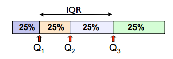
图片来源：Lecture 2: Descriptive Statistics and Exploratory Data Analysis

The first quartile, $ Q_1 $, is the value for which 25% of the observations are smaller and 75% are larger
$ Q_2 $ is the same as the median (50% are smaller, 50% are larger)
Only 25% of the observations are greater than the third quartile $ Q_3 $
IQR, interquartile range, is the difference between the third and the first quartiles, i.e. $ IQR = Q_3 - Q_1 $

这里顺带再图示一下 boxplot 的意思：

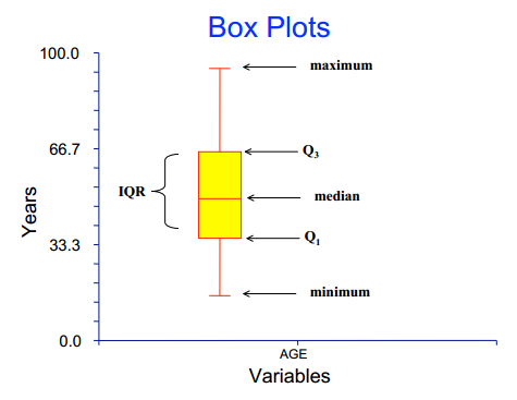
图片来源：Lecture 2: Descriptive Statistics and Exploratory Data Analysis

是不是很清楚？简直一目了然。

另外还有几个别名也提一下：

minimum 到 $ Q_1 $ 的区域也叫 lower whisker
$ Q_3 $ 到 maximum 的区域也叫 upper whisker
minimum 也叫 lower whisker end
maximum 也叫 upper whisker end
$ Q_1 $ 也叫 lower hinge [hɪndʒ]
$ Q_3 $ 也叫 upper hinge

最后注意一种表达方式：quantile a.k.a percentile，在 Week 3 Quiz 的 Question 2 中问到了 “What are the $30^{th}$ and $80^{th}$ quantiles of the resulting data?”，其实就是 $ u_{30\%} $ 和 $ u_{80\%} $，当然我更习惯写成 $ u_{0.30} $ 和 $ u_{0.80} $

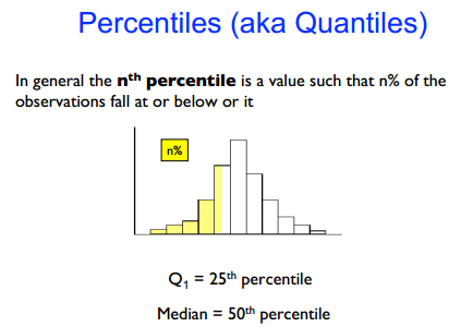
图片来源：Lecture 2: Descriptive Statistics and Exploratory Data Analysis

3.2.3 `table`

table 的作用其实是统计取值的个数，比如：

> table(restData$councilDistrict, useNA="ifany") ## useNA="ifany" 表示如果有 NA，也会计算 NA 的个数；不指定的话，NA 值是不会被统计的

  1   2   3   4   5   6   7   8   9  10  11  12  13  14 
312  85  32  30  40  36  62  18  75 172 277  89  45  54

1 对应的 312 表示 restData$councilDistrict == 1 的有 312 个（i.e. 312 rows）。

同理有二维的 table：

> table(restData$councilDistrict, restData$policeDistrict)
    
     CENTRAL EASTERN NORTHEASTERN NORTHERN ......
  1        0       0            0        0 ......
  2        0       2           27        0 ......
  3        0       0           32        0 ......
  4        0       0            2       28 ......
  ......

2 和 NORTHEASTERN 对应的 27 表示 restData$councilDistrict == 2 && restData$policeDistrict == NORTHEASTERN 的有 27 个（i.e. 27 rows）。

3.2.4 Checking NA

## You can use the complete.cases() function on a data frame, matrix, or vector, which returns a logical vector indicating which cases are complete, i.e., they have no missing values.
## 我们称 a row is complete when it has no NA values
> table(complete.cases(restData)) 

TRUE 
1327

sum(is.na(restData$councilDistrict)) ## 统计 NA 的数量
any(is.na(restData$councilDistrict)) ## 检查 is.na(df$A) 是否有为 TRUE 的，如果有，返回 TRUE；如果是全 FALSE，返回 FALSE
all(restData$zipCode > 0) ## 返回 TRUE / FALSE

> colSums(is.na(restData)) ## is.na(restData) 返回一个 TRUE / FALSE 的 data frame，而且 column 名字还没变，所以接着用 colSums 正好可以统计各个 column 为 is.na 为 TRUE 的数量
  name  zipCode  neighborhood  councilDistrict  policeDistrict  Location.1 
  0     0        0             0                0               0

注意 colSums 是带 column name 的，但是 rowSums 不带，只返回一个 1xn 的 vector。

all(colSums(is.na(restData)) == 0) ## 当 column 太多时，colSums 看起来也不方便，这时用 all 就好了

有点粗暴的处理手段：`na.omit`

na.omit: 去掉有 NA 的行

> DF <- data.frame(x = c(1, 2, 3), y = c(0, 10, NA))
> na.omit(DF)
  x  y
1 1  0
2 2 10

但是要注意，na.omit(DF) 并没有改变 DF 的值，要想改变 DF 的值，需要重新赋值 DF <- na.omit(DF)。

一行内，哪怕只要有一个 NA，这一行也会被 na.omit 直接干掉。所以很有必要计算下干掉的行数的比例，比如你一下干掉 50% 的行数，这肯定是不妥的，这时就要转入 impute 程序。

3.2.5 Checking values with specific characteristics: 统计某单个变量的取值 (`%in%` and `unique`)

没啥好说的，注意 %in% 的用法就好（类似于 collection.contains(obj) 操作）。

> table(restData$zipCode %in% c("21212"))

FALSE  TRUE 
 1299    28 
> table(restData$zipCode %in% c("21212","21213"))

FALSE  TRUE 
 1268    59 
> restData[restData$zipCode %in% c("21212","21213"),]
                 name zipCode                neighborhood councilDistrict policeDistrict ......
29  BAY ATLANTIC CLUB   21212                    Downtown              11        CENTRAL ......
39  BERMUDA BAR         21213               Broadway East              12        EASTERN ......
92  ATWATER'S           21212   Chinquapin Park-Belvedere               4       NORTHERN ......
......

然后 unique 可以排除重复元素：

> x <- c(1:5, 2:6)
> unique(x)
[1] 1 2 3 4 5 6

3.2.6 Cross Tabulation (`xtabs`): 统计多个变量的取值组合

这次换个小点的数据集来演示：

data(UCBAdmissions) ## BTW, data() will show you a list of data sets within R
df = as.data.frame(UCBAdmissions)
summary(df)

##      Admit       Gender   Dept       Freq      
##  Admitted:12   Male  :12   A:4   Min.   :  8.0  
##  Rejected:12   Female:12   B:4   1st Qu.: 80.0  
##                            C:4   Median :170.0  
##                            D:4   Mean   :188.6  
##                            E:4   3rd Qu.:302.5  
##                            F:4   Max.   :512.0

> xtabs(Freq ~ Gender + Admit, data=df)
        Admit
Gender   Admitted Rejected
  Male       1198     1493
  Female      557     1278

这个表的意思是：满足 Gender=="Male" & Admit=="Admitted" 的所有 row 的 Freq 的和为 1198；依次类推。

我们可以自行验证一下：

> df[df$Gender=="Male" & df$Admit=="Admitted", ]
      Admit Gender Dept Freq
1  Admitted   Male    A  512
5  Admitted   Male    B  353
9  Admitted   Male    C  120
13 Admitted   Male    D  138
17 Admitted   Male    E   53
21 Admitted   Male    F   22
> sum(df[df$Gender=="Male" & df$Admit=="Admitted", ]$Freq)
[1] 1198

当 xtabs 超过 2 维时，输出就有点难看了，这时可以用 ftable 来调整下输出的格式：

> xt <- xtabs(Freq ~ ., data=df)
> ftable(xt)
                Dept   A   B   C   D   E   F
Admit    Gender                             
Admitted Male        512 353 120 138  53  22
         Female       89  17 202 131  94  24
Rejected Male        313 207 205 279 138 351
         Female       19   8 391 244 299 317

注意一定要 ftable(xtab) 套用才行，直接 ftable(Freq ~ ., data=df) 的输出也是很长很散的。

3.2.7 Calculating the size of a dataset

> object.size(df)
3216 bytes
> print(object.size(df), units="Kb")
3.1 Kb
> print(object.size(df), units="Mb")
0 Mb

3.3 Adding New Variables (i.e. New Columns)

3.3.1 How to add columns and rows

> df <- data.frame(A=1:3, B=4:6, C=7:9) ## 原始 df

> df <- cbind(df, 10:12) ## 添加一个 column，但是 column name 会直接变成 "10:12"

> D <- 10:12
> df <- cbind(df, D) ## 新 column name 为 D

> df$D <- 10:12 ## 更直接的方式

> df <- rbind(df, rep(0, 3)) ## add a row

这里要强调一下：cbind 多个 vector 产生的是 matrix 而不是 data frame。之所以强调这一点是因为有些 generic function (比如 melt) 会根据实际的参数类型来选择不同的操作。

根据 Creating a data frame from two vectors using cbind：

cbind(A=1:3, B=4:6) 是 matrix
data.frame(A=1:3, B=4:6) 是 df
cbind.data.frame(A=1:3, B=4:6) 是 df
cbind(df, C=7:9) 是 df

另外，添加 column 后总会有调整 column 顺序的需求，而且一般都是把 last column 往前排，这里介绍一种比较简单的方法：

data[, c(ncol(data),1:(ncol(data)-1))] ## move last column to first
data[, c(1,ncol(data),2:(ncol(data)-1))] ## move last column to second
data[, c(1:2,ncol(data),3:(ncol(data)-1))] ## move last column to third

## 发现规律了么？

3.3.2 Creating mathematical variables

abs(x): absolute value
sqrt(x): square root
ceiling(x): e.g. ceiling(3.475) == 4
floor(x): e.g. floor(3.475) == 3
trunc(x): 截取整数部分，e.g. trunc(-5.99) == -5
round(x, digits=n): rounds to ‘n’ decimal places (default 0) (保留 n 位小数). e.g. round(3.475, digits=2) == 3.48
signif(x, digits=n): rounds to ‘n’ significant digits (保留 n 位有效数字). e.g. signif(3.475, digits=2) == 3.5
cos(x), sin(x) etc.
log(x): natural logarithm, i.e. $ \log_e x $, a.k.a $ \ln x $
log2(x): $ \log_2 x $
log10(x): $ \log_{10} x $, a.k.a $ \lg x $
exp(x): exponentiating x, i.e. e^x
sd(x): takes the standard deviation of x
range(x): displays the range; same as c(min(x), max(x))
x - mean(x): centering x
(x - mean(x)) / sd(x): 计算 x 的 z-score

3.3.3 Creating sequences or indices

用 seq 创建好再添加为新 column 就可以了：

> seq(1, 10, by=2) ## sequence increases by 2
[1] 1 3 5 7 9

> seq(1, 10, length=3) ## create a sequence whose length is 3
[1]  1.0  5.5 10.0

> x <- c(1,3,8,25,100) ## create a sequence along x
seq(along = x)
[1] 1 2 3 4 5

3.3.4 Adding subset result

其实就是把 subset 的结果添加为新 column：

restData$nearMe <- restData$neighborhood %in% c("Roland Park", "Homeland")

还有一种 ifelse 操作，十分类似 Java 的三目运算符 ? ::

restData$zipState <- ifelse(restData$zipCode < 0, "invalid", "valid") ## restData$zipCode < 0? "invalid" : "valid"

这个 Java 一样，也是可以嵌套的，比如：

ALevels = ifelse(df$A < 10000, "low", ifelse(df$A > 20000, "high", "med"))

3.3.5 Creating categorical variables

3.3.5.1 Creating factor variables

根据 column 直接生成一个 factor 是很简单的，直接把 column 传给 factor() 就可以了：

restData$zcf <- factor(restData$zipCode)

有时候需要特别指定一下 levels：

> yesno <- sample(c("yes","no"), size=10, replace=TRUE)
> factor(yesno) ## 默认情况下，levels 按字母顺序排列，所以 no 是 level#1，yes 是 level#2
 [1] no  no  yes yes no  yes yes yes no  no 
Levels: no yes
> factor(yesno, levels=c("yes","no")) ## 这里指定 levels=c("yes","no") 的话，那 yes 就是 level#1，no 是 level#2
 [1] no  no  yes yes no  yes yes yes no  no 
Levels: yes no

也可以用 relevel：

> yesnofac <- factor(yesno)
> yesnofac
 [1] no  no  yes yes no  yes yes yes no  no 
Levels: no yes
> yesnofac <- relevel(yesnofac, ref="yes") ## relevel 的作用是把 ref 提到 level#1，ref 之前的 levels 顺序往后挪一位。factor 本身的元素顺序并不受影响
## 另外要注意 relevel 并不会改变 yesnofac 本身，所以还是要再次赋个值
> yesnofac
 [1] no  no  yes yes no  yes yes yes no  no 
Levels: yes no

这里要提一下，relevel 会影响 as.numeric(factor) 的值：

> as.numeric(factor(yesno))
 [1] 1 1 2 2 1 2 2 2 1 1
> as.numeric(relevel(factor(yesno), ref="yes"))
 [1] 2 2 1 1 2 1 1 1 2 2

可见 as.numeric() 的值是就是 level#，你是 level#1，那值就为 1，和 level#1 具体是什么没有关系。

3.3.5.2 Cutting values into categories

Using `cut` function

还是用 3.2 Summarizing Data 的试验数据。先看一个例子：

> quantile(restData$councilDistrict)
  0%  25%  50%  75% 100% 
   1    2    9   11   14 

> restData$councilDistrictGroup <- cut(restData$councilDistrict, breaks=quantile(restData$councilDistrict), include.lowest=TRUE)
> restData$councilDistrictGroup
   [1] [1,2]   [1,2]   [1,2]   (11,14] (2,9]   (11,14] (11,14] (2,9]  
   [9] (11,14] [1,2]   (9,11]  (2,9]   [1,2]   [1,2]   (9,11]  (9,11] 
  [17] (11,14] [1,2]   [1,2]   (9,11]  [1,2]   (9,11]  (2,9]   [1,2] 
......
[1321] (11,14] (9,11]  (2,9]   [1,2]   (11,14] (2,9]   [1,2] 
Levels: [1,2] (2,9] (9,11] (11,14]

> table(restData$councilDistrictGroup)

  [1,2]   (2,9]  (9,11] (11,14] 
    397     293     449     188

cut 简单说就是按 breaks 的区间来分组：

如果 breaks = n，那就是分 n 个组
如果 breaks = c(x, y, z)，那就是分 (x, y], (y, z] 这么两个组，依此类推

这里我们 breaks=quantile()，所以分组是 (1, 2]、(2, 9]、(9, 11]、(11, 14]，然后我们加了一个 include.lowest=TRUE，于是第一个分组就变成了 [1, 2]。这么做也是因为 quantile 里说过 “理论上 $ u_{0.00} $ 不应该是 1”，不设置 include.lowest=TRUE 的话，restData$councilDistrict == 1 的 row 的 councilDistrictGroup 就是 NA。

你应该已经注意到了，cut 得到的结果是一个 factor，其实还可以指定 labels=c("low", "below median", ...) 来设置这个 factor 的 levels（注意 quantile 产生了 5 个值，但是只有 4 个区间，所以 labels 的长度也是 4）。如果直接设置 labels=FALSE，那么 cut 得到的结果就不再是一个 factor，而是一个 vector，若属于第一个分组，那么值就为 1，依此类推。

Easier cutting (with `cut2`)

> library(Hmisc)
> restData$councilDistrictGroup <- cut2(restData$councilDistrict, g=4) ## g=4 表示分 4 个 group
> table(restData$councilDistrictGroup)

[ 1, 3) [ 3,10) [10,12) [12,14] 
    397     293     449     188

注意分组区间的开闭。结果和前面 cut(include.lowest=TRUE) 的恰好一致。

Using `mutate` function

mutate 就是 “基因突变” “变异” 的那个意思，注意下用法就好了，和直接加 column 差不多：

library(Hmisc); 
library(plyr);
restData2 <- mutate(restData, zipGroups=cut2(zipCode,g=4)) ## 作用是：以 restData 为基础，添加一个名为 zipCode 的 column，值为 cut2(zipCode,g=4)
## mutate 并不会改变 restData 的值

3.4 Reshaping Data

3.4.1 Melting data frames

melt 是一个 generic function，它会根据实际的参数类型来确定具体调用哪个 melt 方法：

melt.data.frame for data.frames
melt.array for arrays, matrices and tables
melt.list for lists

这里我们只演示 data frame 的情况：

> library(reshape2)
> df <- data.frame(A=1:3, B=4:6, C=7:9, D=10:12)
> df <- rbind(df, c(4, NA, NA, 13))
> df
  A  B  C  D
1 1  4  7 10
2 2  5  8 11
3 3  6  9 12
4 4 NA NA 13
> mdf <- melt(df, id=c("A"), measure.vars=c("B", "C", "D"), na.rm=TRUE) ## remove NA of the molten result from row 4 
> mdf[order(mdf$A),]
   A variable value
1  1        B     4
5  1        C     7
9  1        D    10
2  2        B     5
6  2        C     8
10 2        D    11
3  3        B     6
7  3        C     9
11 3        D    12
12 4        D    13

初看有点难理解。在 Reshaping data with the reshape package 里有说，melt 的作用是：

… represent this data set…, where each row represents one observation of one variable.

可以考虑这样一种场景，A 是病人 id，B、C、D 这些是体检项目，第一行 (1, 4, 7, 10) 表示 “1 号病人三项体检的数据分别是 4、7、10”。第四行 (4, NA, NA, 13)，表示 “4 号病人只进行了 D 体检，数据是 13”。

我们用 melt 之后，每一行就只显示单个病人单项体检的数据了。

不管你如何设置，固定的效果是多出 variable 和 value 这两个 column。

再说一下参数：

id: id variables，可以有多个，你可以理解成联合主键
measure.vars: 其实应该是 measured variables。不一定要把 id 之外的 var 都用上，比如前面那个例子，如果你不关心体检 D 的数据，你设置 measure.vars=c(“B”, “C”) 就可以了

再介绍一些写法惯例：

melt(df) ## 所有的 var (column) 都是 measure.vars，系统自己分配 id
melt(df, id=c("A")) ## 自动把 A 以外的所有 var 设置成 measure.vars
melt(df, measure.vars=c("B", "C", "D")) ## 自动把剩下 A 设置成 id
melt(df, id=1:2) ## 把第一项（A）和第二项（B）设置成 id，剩下的 var 设置成 measure.vars

3.4.2 Casting data frames

cast 最直观的作用就是把 melt 的结果重新拼回来，分为 acast 和 dcast 两种，功能和用法是一样的，只是返回不同

dcast 返回 data frame
acast 返回 array (matrix)

我们这里只演示 dcast：

> library(reshape2)
> df <- data.frame(A=1:3, B=4:6, C=7:9, D=10:12)
> df <- rbind(df, c(4, NA, NA, 13))
> mdf <- melt(df, id=c("A"), measure.vars=c("B", "C", "D"), na.rm=TRUE)
> mdf
   A variable value
1  1        B     4
2  2        B     5
3  3        B     6
5  1        C     7
6  2        C     8
7  3        C     9
9  1        D    10
10 2        D    11
11 3        D    12
12 4        D    13 
> dcast(mdf, A ~ variable)
  A  B  C  D
1 1  4  7 10
2 2  5  8 11
3 3  6  9 12
4 4 NA NA 13

注意这里是简写，完整一点的写法是：dcast(mdf, A ~ variable, value.var=c("value"))，只是 dcast 存在一个自动识别 value.var 的机制（guess_value 函数）：

Is value or (all) column present? If so, use that

Otherwise, guess that last column is the value column

这个 “or (all)” 十分 confusing，直到我看到了 guess_value 的源码。我不禁想吼一句：尼玛用个引号引一下会死啊！所以这里实际是：

value.var=c("value") or value.var=c("(all)"), if any
Otherwise, use the last column

cast 的结果就是把 “each row represents one observation of one variable” 变回 “each row represents one observation”，X ~ Y 的 Y 的值都变成了 variable，而这些 variable 的值由 value.var 这个 column 来填充。

formula 也可以有多项的情况，写法为 X1 + X2 ~ Y1 + Y2，这时 Y1 和 Y2 的值的组合（用下划线连接，foo_bar 这样）会变成 variable。

下面说下 . 和 ...:

. corresponds to no variable
... represents all variables not previously included in the casting formula. Including this in your formula will guarantee that no aggregation occurs. There can be only one ... in a cast formula.

这里用原始的 df 直接演示下（这也说明 cast 不一定非要用在 melt 的结果上）：

> df <- data.frame(A=1:3, B=4:6, C=7:9, D=10:12)
> df
  A B C  D
1 1 4 7 10
2 2 5 8 11
3 3 6 9 12
> dcast(df, A ~ .) ## 只有病人 id，没有体检项目
Using D as value column: use value.var to override.
  A  .
1 1 10
2 2 11
3 3 12
> dcast(df, . ~ A) ## 没有病人 id，体检项目是 A 的值
Using D as value column: use value.var to override.
  .  1  2  3
1 . 10 11 12
> dcast(df, A ~ ...) ## all variables except A and value.var (D)，所以是 B 和 C，但是要注意是 B+C
Using D as value column: use value.var to override.
  A 4_7 5_8 6_9
1 1  10  NA  NA
2 2  NA  11  NA
3 3  NA  NA  12
> dcast(df, ... ~ A) ## all variables except A and value.var (D)，所以是 B 和 C，要注意的是 B+C 写在 formula 左端是不像写在右端那样会组合 B_C 的
Using D as value column: use value.var to override.
  B C  1  2  3
1 4 7 10 NA NA
2 5 8 NA 11 NA
3 6 9 NA NA 12

上面还提到了 aggregation，这里其实有一个非常重要的规则：

fun.aggregate: aggregation function needed if variables do not identify a single observation for each output cell. Defaults to length (with a message) if needed but not specified.

这里实际的意思是：如果 formula 左端的 id 不能唯一确定一行（i.e. a single observation）时，所有的 id 会实际对应一个 observation 列表，dcast 会在列表上执行 fun.aggregate 参数指定的 function，默认是 length。举个例子看看：

> df2 <- rbind(df, c(1, 13, 14, 15))
> df2
  A  B  C  D
1 1  4  7 10
2 2  5  8 11
3 3  6  9 12
4 1 13 14 15
> dcast(df2, A ~ .)
Using D as value column: use value.var to override.
Aggregation function missing: defaulting to length
  A .
1 1 2 ## 表示 A = 1 的有两个 observation
2 2 1
3 3 1

这个功能拿来做统计其实很有用：

> dcast(df2, A ~ ., fun.aggregate=sum)
Using D as value column: use value.var to override.
  A  .
1 1 25
2 2 11
3 3 12
> dcast(df2, A ~ ., fun.aggregate=mean)
Using D as value column: use value.var to override.
  A    .
1 1 12.5
2 2 11.0
3 3 12.0

最后介绍下两个参数 margins 和 subset。

margins 这个描述起来有点困难，可以看下面代码的例子。目前已知 margins 取值可以是 formula 右边的任意一个 column 或者多个 column 的组合，或者直接 margins=TRUE 表示 all possible margins。文档里提到的 “grand_col” 和 “grand_row” 应该是 obsolete 了，至少我在源码里没见着。

## 对于 A ~ B + C，margins 可以取 "B" 或 "C" 或者 c("B", "C")
> dcast(df2, A ~ B + C, sum, margins="B")
> dcast(df2, A ~ B + C, sum, margins="C")
> dcast(df2, A ~ B + C, sum, margins=c("B", "C"))
> dcast(df2, A ~ B + C, sum, margins=TRUE)
Using D as value column: use value.var to override.
      A 4_7 4_(all) 5_8 5_(all) 6_9 6_(all) 13_14 13_(all) (all)_(all)
1     1  10      10   0       0   0       0    15       15          25
2     2   0       0  11      11   0       0     0        0          11
3     3   0       0   0       0  12      12     0        0          12
4 (all)  10      10  11      11  12      12    15       15          48

这个效果看自己体会一下吧，有点难解释。

subset 这个简单点，表示 “dcast 应该在 data frame 的 subset 上进行”。subset 的值为 subsetting 的条件，但是要注意写法：

> library(plyr)
> dcast(df2, A ~ ., sum)
Using D as value column: use value.var to override.
  A  .
1 1 25
2 2 11
3 3 12
> dcast(df2, A ~ ., sum, subset=.(A<3)) ## this `.` requires plyr. in fact, `.` is a function
Using D as value column: use value.var to override.
  A  .
1 1 25
2 2 11

3.4.3 Calculate on groups

这一小节 slide 上是叫 “Averaging Values”，但是给的例子又是 sum 操作……其实就是这篇 A quick primer on split-apply-combine problems 里说的 split-apply-combine problems，也就是：

I want to calculate some statistic for lots of different groups.

我们掌握下函数的用法就好了。以分组 sum 为例：

> tapply(InsectSprays$count, InsectSprays$spray, sum)
  A   B   C   D   E   F 
174 184  25  59  42 200 

## 效果上它等价于：
> s <- split(InsectSprays$count, InsectSprays$spray)
> lapply(s, sum) ## 但是返回结果是 list
## or
> sapply(s, sum) ## 返回结果简化成 vector
## or 
> unlist(lapply(s, sum)) ## to convert a list to vector (with column name)

如果用 plyr 的话可以用：

> library(plyr)
> ddply(InsectSprays, .(spray), summarize, sum=sum(count))
  spray sum
1     A 174
2     B 184
3     C  25
4     D  59
5     E  42
6     F 200

## 先将 InsectSpray 按 .(spray) 分组，然后在每个分组上执行 summarize，summarize 的参数是 sum=sum(count)
## 分组结果可以用 ddply(InsectSprays, .(spray), print) 查看

如果想把分组 sum 添加到 data frame，可以用：

> spraySums <- ddply(InsectSprays, .(spray), summarize, sum=ave(count,FUN=sum))
> head(spraySums)
  spray sum
1     A 174
2     A 174
3     A 174
4     A 174
5     A 174
6     A 174
## ave 的作用是在指定的列（或者列的 subset）上执行 FUN（默认是 mean），然后将计算结果附到该列的每个值的后面

Using `aggregate` function

简单举个例子：

aggregate(. ~ cyl + gear, data=mtcars, FUN=mean)

这一句的意思是：

group all the other variables (“.” means “all the other variables not appeared in this formula”) in mtcars by cyl and gear
apply mean to all the groups

有几点需要注意：

这里 mean 的效果其实是 colMeans(group)
最后得到的 data frame 的 column 没有变化，只是 cyl 和 gear 提前了
row.names(mtcars) 是车名，aggregate 结果的 row.names 是 “1” “2” “3” “4” “5” “6” “7” “8”

3.5 Merging Data

数据准备：

if(!file.exists("./data")){dir.create("./data")}
fileUrl1 = "http://dl.dropboxusercontent.com/u/7710864/data/reviews-apr29.csv"
fileUrl2 = "http://dl.dropboxusercontent.com/u/7710864/data/solutions-apr29.csv"
download.file(fileUrl1,destfile="./data/reviews.csv",method="auto")
download.file(fileUrl2,destfile="./data/solutions.csv",method="auto")
reviews = read.csv("./data/reviews.csv"); 
solutions = read.csv("./data/solutions.csv")

3.5.1 Using `merge`

mergedData = merge(reviews, solutions, by.x="solution_id", by.y="id", all=TRUE)

这个学过数据库的应该很了解了（参 join）：

all=TRUE 表示 all.x=TRUE & all.y=TRUE
- all.x=TRUE 表示 x 中的所有 row （包括不匹配的）都会进入 merge 后的表，对应的 y 的 column 值被填成 NA。其实就是 Left Out Join
- all.y=TRUE 就是 Right Out Join
all=TRUE 就是 Full Outer Join

不指定 by.x 或者 by.y 的话，merge all common column names

3.5.2 Using `join` in the `plyr` package

Faster, but less full featured. Defaults to left join, see help file for more.

df1 = data.frame(id=sample(1:10), x=rnorm(10))
df2 = data.frame(id=sample(1:10), y=rnorm(10))
arrange(join(df1,df2), id) ## arrange 的作用是把行号和 id 都排列整齐
   id       x       y
1   1  0.2514  0.2286
2   2  0.1048  0.8395
3   3 -0.1230 -1.1165
4   4  1.5057 -0.1121
5   5 -0.2505  1.2124
6   6  0.4699 -1.6038
7   7  0.4627 -0.8060
8   8 -1.2629 -1.2848
9   9 -0.9258 -0.8276
10 10  2.8065  0.5794

3.5.3 Using `join_all` if you have multiple data frames

df1 = data.frame(id=sample(1:10), x=rnorm(10))
df2 = data.frame(id=sample(1:10), y=rnorm(10))
df3 = data.frame(id=sample(1:10), z=rnorm(10))
dfList = list(df1, df2, df3)
arrange(join_all(dfList), id)
   id          x          y           z
1   1  2.0960882  0.6083729  1.48008618
2   2  0.2118634 -0.6795807 -0.59807800
3   3  2.1070553  1.7892524  1.09027314
4   4  0.2200364 -0.5269966  0.34988603
5   5 -2.6525629 -0.3318976 -0.02793177
6   6  0.5124324 -1.0701264 -0.25701533
7   7  0.3555252 -0.2692719 -0.41907259
8   8  1.3038877 -1.3293329  1.12601196
9   9  0.8370239 -0.5411611  2.34161938
10 10 -0.3579197 -0.8578622  1.57283904

3.5.4 Using `stack` to combine vectors

You have several vectors and you want to combine these vectors into a large one and simultaneously create a parallel factor that identifies each value’s origin.

Create a list that contains the vectors. Then use the stack function to combine the list into a two-column data frame:

The values column contains the data
The ind column contains the parallel factor

举个例子就好懂了：

freshmenGrade = c(90,85,80)
sophomoresGrade = c(88,82,91)
juniorsGrade = c(78,93,95)

allGrade = stack(list(fresh=freshmenGrade, soph=sophomoresGrade, jrs=juniorsGrade))
allGrade
  values   ind
1     90 fresh
2     85 fresh
3     80 fresh
4     88  soph
5     82  soph
6     91  soph
7     78   jrs
8     93   jrs
9     95   jrs

3.6 Editing Text Variables

3.6.1 Important points about text in data sets

Names of variables should be
- All lower case when possible
- Descriptive (Diagnosis versus Dx)
- Not duplicated
- Not have underscores or dots or white spaces

Variables with character values
- Should usually be made into factor variables (depends on application)
- Should be descriptive (use TRUE/FALSE instead of 0/1 and Male/Female versus 0/1 or M/F)

3.6.2 Best practices of processsing variable names

准备数据：

if(!file.exists("./data")){dir.create("./data")}
fileUrl <- "http://data.baltimorecity.gov/api/views/dz54-2aru/rows.csv?accessType=DOWNLOAD"
download.file(fileUrl,destfile="./data/cameras.csv",method="auto")
cameraData <- read.csv("./data/cameras.csv")

Make lower case when possible

names(cameraData)
names(cameraData) <- tolower(names(cameraData)) ## BTW, toupper() makes it upper case

Delete suffix “.1” like in “Location.1”

> splitNames = strsplit(names(cameraData),"\\.")
> splitNames[[6]]
[1] "Location" "1"
> splitNames = sapply(splitNames, function(x) { x[1] })
> splitNames
[1] "address"      "direction"    "street"       "crossStreet" 
[5] "intersection" "Location"

Delete underscore

> v <- c("A", "B", "C_1")
> v1 <- sub("_", "", v) ## sub for substitute
> v1
[1] "A"  "B"  "C1"

> v <- c("A", "B", "C_1_1")
> v2 <- sub("_", "", v1) ## 但是 sub 只能替换第一个遇到的 `_`
> v2
[1] "A"    "B"    "C1_1"

> v2 <- gsub("_", "", v) ## 使用 gsub 替换全部 `_`
> v2
[1] "A"   "B"   "C11"

Rename a single column

> names(df)[names(df) == 'old.var.name'] <- 'new.var.name'

3.6.3 `grep` and `grepl`

> grep("Alameda", cameraData$intersection) ## 返回 index
[1]  4  5 36
> grep("Alameda", cameraData$intersection, value=TRUE) ## 返回匹配的 item
[1] "The Alameda  & 33rd St"   "E 33rd  & The Alameda"   
[3] "Harford \n & The Alameda"
> grepl("Alameda", cameraData$intersection) ## l for "logical vector"
 [1] FALSE FALSE FALSE  TRUE  TRUE FALSE FALSE FALSE FALSE FALSE FALSE FALSE
[13] FALSE FALSE FALSE FALSE FALSE FALSE FALSE FALSE FALSE FALSE FALSE FALSE
[25] FALSE FALSE FALSE FALSE FALSE FALSE FALSE FALSE FALSE FALSE FALSE  TRUE
[37] FALSE FALSE FALSE FALSE FALSE FALSE FALSE FALSE FALSE FALSE FALSE FALSE
[49] FALSE FALSE FALSE FALSE FALSE FALSE FALSE FALSE FALSE FALSE FALSE FALSE
[61] FALSE FALSE FALSE FALSE FALSE FALSE FALSE FALSE FALSE FALSE FALSE FALSE
[73] FALSE FALSE FALSE FALSE FALSE FALSE FALSE FALSE
> table(grepl("Alameda", cameraData$intersection)) ## 查看匹配与否的数量

FALSE  TRUE 
   77     3 
> grep("JeffStreet", cameraData$intersection)
integer(0)
> grep("JeffStreet", cameraData$intersection, value=TRUE)
character(0)
> length(grep("JeffStreet", cameraData$intersection)) ## 判断是否有匹配
[1] 0

## 根据匹配与否来 subset
> cameraData2 <- cameraData[grep("Alameda", cameraData$intersection), ]
> cameraData3 <- cameraData[!grepl("Alameda",cameraData$intersection), ]

3.6.4 Some other String functions

> library(stringr)
> nchar("Jeffrey Leek") ## 相当于 Java 的 String.length(); R 的 length() 是返回 vector 或者 list 的元素个数，不要误用
[1] 12

> nchar(c("Moe", "Larry", "Curly")) ## nchar 也可以用于 string vector
[1] 3 5 5

> substr("Jeffrey Leek", 1, 7)
[1] "Jeffrey"

> substr(c("Moe", "Larry", "Curly"), 1, 3) ## Extract first 3 characters of each string
[1] "Moe" "Lar" "Cur"

> cities <- c("New York, NY", "Los Angeles, CA", "Peoria, IL") 
> substr(cities, nchar(cities)-1, nchar(cities)) ## In fact, all the arguments can be vectors, in which case substr will treat them as parallel vectors
[1] "NY" "CA" "IL"

> paste("Jeffrey", "Leek") ## 注意拼接结果自带一个空格
[1] "Jeffrey Leek"
> paste("Hello", "world", sep=",")
[1] "Hello,world"
> paste0("foo", "bar") ## 不会带空格
[1] "foobar"

> paste("Visit", 1:5, sep = "_")
[1] "Visit_1" "Visit_2" "Visit_3" "Visit_4" "Visit_5"
> paste("Visit", 1:5, sep = "_", collapse = " ") ## collapse is used to separate the results
[1] "Visit_1 Visit_2 Visit_3 Visit_4 Visit_5"

> library(stringr)
> str_trim("foo   ")
[1] "foo"

> id <- c(1, 2, 3)
> formatC(id, width=3, flag="0") ## 格式化输出：将 id 输出为长度为 3 的串，不够长的填 0
[1] "001" "002" "003"

3.6.5 Regular Expressions

Regular Expression has 2 components:

literals: keywords，一个词，比如 “foo”
- Simplest pattern consists only of literals
- A match occurs if the sequence of literals occurs anywhere in the text being tested
metacharacters are used to express:
- whitespace word boundaries
- sets of literals
- the beginning and end of a line
- alternatives (“foo” or “bar”)

^i think: match lines starting with “i think”
morning$: match lines ending with “morning” or we can say $ represents the end of a line
[Ff][Oo][Oo]: 匹配 FOO, FOo, FoO, Foo, fOO, fOo, foO, foo；注意这种形式是可以匹配 xxFOOzz 这样字符串的，因为我们并没有指定 [Ff][Oo][Oo] 是匹配一个完整的词
^[Ii] am: match lines starting with “I am” or “i am”
^[0-9][a-zA-Z]: 匹配 “1 数字 1 字母” 模式，比如 “7th” 里的 “7t”
[^?.]$: anything other than “?” or “.” at the end of a line；注意这个语法，[?.] 表示 “?” or “.”，前面加个 ^ 表示否定，就是 not “?” or “.”

.: is used to refer to any single character，比如 3.21 可以匹配 3-21, 3/21, 203.219, 03:21, 3321 等
- 但是 . 在 [] 里是直接表示句号的，连转义也不需要
- .*: 匹配任意多个字符
- (.*): 匹配括号内的任意多个字符
flood|fire: “flood” or “fire”, matching e.g. firewire, floods
^[Gg]ood|[Bb]ad: 注意 ^ 只作用于 [Gg]ood
^([Gg]ood|[Bb]ad): 这样 ^ 就同时起作用了
[Gg]eorge( [Ww]\.)? [Bb]ush: 可以匹配 George W. Bush, George Bush 等
- (xxx)? indicates that the expression “xxx” is optional（对单个字符可以不用括号，比如 AB?C）
- \. 是转义
[0-9]+: 任意一个或多个数字
[Bb]ush( +[^ ]+ +){1,5} debate: 首先看中间那个括号，+个空格，然后+个非空格，再+个空格。然后这整个括号的结构可以重复 1-5 次。简单说就是 bush 和 debate 之间可以有 1-5 个单词，这 1-5 个单词之间可以有+个空格
- {5}: 表示 exactly 重复 5 次
- {1,}: 表示重复 at least 1 次
　+([a-zA-Z]+) +\1+: +个空格（注意：开头的这个空格我用的是全角，用半角的话会被吞掉），接着\+个字母，再\+个空格，然后 `\1` 表示与前面括号内的匹配内容一样（这种用法仅限于引用括号的匹配内容），也是\+个。简单说就这就用来匹配两个相同的单词的，比如 " foo foo"

The * is “greedy” so it always matches the longest possible string that satisfies the regular expression.
- 比如 ^s(.*)s 会匹配整个 “sitting at starbucks”，而不是 “sitting at s”
- The greediness of * can be turned off with the ?, as in ^s(.*?)s$

3.6.6 Working with Dates

> d1 = date()
> d1
[1] "Tue Aug 12 14:58:40 2014"
> class(d1)
[1] "character"
> d2 = Sys.Date()
> d2
[1] "2014-08-12"
> class(d2)
[1] "Date"

> format(d2,"%a %b %d")
[1] "周二 八月 12"

%d = day as number (01-31)
%a = abbreviated weekday
%A = unabbreviated weekday
%m = month (01-12)
%b = abbreviated month
%B = unabbrevidated month
%y = 2-digit year
%Y = 4-digit year

For more format, click Date Formats in R.

> Sys.setlocale("LC_TIME", "C");
> x = c("1jan1960", "2jan1960", "31mar1960", "30jul1960")
> z = as.Date(x, "%d%b%Y")
> z
[1] "1960-01-01" "1960-01-02" "1960-03-31" "1960-07-30"
> z[1] - z[2]
Time difference of -1 days
> as.numeric(z[1]-z[2])
[1] -1

这里就 locale 说两句：

这里 “LC_TIME” 和 “C” 是 *nix 的概念，并不是 R 特有的。设置 “LC_TIME” 为 “C” 表示 “use the default locale for LC_TIME”，具体可以参见 What does “LC_ALL=C” do?
可以用 strsplit(Sys.getlocale(), ";") 来查看当前的 locale 信息。strsplit 是为了让输出好看一点~

> weekdays(d2) ## 不能用于 d1
[1] "Tuesday"
> months(d2)
[1] "August"
> julian(d2) ## days since 1970-01-01
[1] 16294
attr(,"origin")
[1] "1970-01-01"
> attr(julian(d2), "origin")
[1] "1970-01-01"

> library(lubridate); 
> ymd("20140108")
[1] "2014-01-08 UTC"
> mdy("08/04/2013")
[1] "2013-08-04 UTC"
> dmy("03-04-2013")
[1] "2013-04-03 UTC"
> ymd_hms("2011-08-03 10:15:03")
[1] "2011-08-03 10:15:03 UTC"
> ymd_hms("2011-08-03 10:15:03", tz="Pacific/Auckland") ## ?Sys.timezone for more information on timezone
[1] "2011-08-03 10:15:03 NZST"
> x = dmy(c("1jan2013", "2jan2013", "31mar2013", "30jul2013"))
> wday(x[1])
[1] 3
> wday(x[1],label=TRUE)
[1] Tues
Levels: Sun < Mon < Tues < Wed < Thurs < Fri < Sat

Twitter Facebook LinkedIn

1. Basis

1.1 Overview

1.2 Definition of Data, Raw Data and Processed Data

1.3 Components of Tidy Data

1.3.1 Standards of Tidy Data Set and Tidy Data Files

1.3.2 The code book

How to code variables

1.3.3 Scripts and Instructions

2. Reading Data

2.1 Downloading Files

2.2 read.table args: na.strings, stringsAsFactors, comment.char

na.strings 参数

stringsAsFactors 参数

comment.char 参数

2.3 The data.table Package

2.3.1 Using tables

2.3.2 Referencing

2.3.3 Calculation inside the data table

2.3.4 Adding new columns

2.3.5 Group by, .N, Keys and Join

Group By

.N

Keys

Join

2.3.6 Fast Reading

2.4 Webscraping

2.5 The sqldf Package

3. Handling Data At The Very Beginning

3.1 Subsetting and Sorting

3.1.1 Subsetting

Using subset function

Using which, which.min, which.max functions

How to remove columns?

Making new data frames by extraction

3.1.2 Sorting

3.1.3 Ordering

3.1.3 Ordering with plyr

3.2 Summarizing Data

3.2.1 dim, nrow, ncol, colnames, head, tail, summary and str

3.2.2 quantile

3.2.3 table

3.2.4 Checking NA

有点粗暴的处理手段：na.omit

3.2.5 Checking values with specific characteristics: 统计某单个变量的取值 (%in% and unique)

3.2.6 Cross Tabulation (xtabs): 统计多个变量的取值组合

3.2.7 Calculating the size of a dataset

3.3 Adding New Variables (i.e. New Columns)

3.3.1 How to add columns and rows

3.3.2 Creating mathematical variables

3.3.3 Creating sequences or indices

3.3.4 Adding subset result

3.3.5 Creating categorical variables

3.3.5.1 Creating factor variables

3.3.5.2 Cutting values into categories

Using cut function

Easier cutting (with cut2)

Using mutate function

3.4 Reshaping Data

3.4.1 Melting data frames

3.4.2 Casting data frames

3.4.3 Calculate on groups

Using aggregate function

3.5 Merging Data

3.5.1 Using merge

3.5.2 Using join in the plyr package

3.5.3 Using join_all if you have multiple data frames

3.5.4 Using stack to combine vectors

3.6 Editing Text Variables

3.6.1 Important points about text in data sets

3.6.2 Best practices of processsing variable names

Make lower case when possible

Delete suffix “.1” like in “Location.1”

Delete underscore

Rename a single column

3.6.3 grep and grepl

3.6.4 Some other String functions

3.6.5 Regular Expressions

3.6.6 Working with Dates

Comments

You May Also Enjoy

2.2 `read.table` args: `na.strings`, `stringsAsFactors`, `comment.char`

`na.strings` 参数

`stringsAsFactors` 参数

`comment.char` 参数

2.3 The `data.table` Package

2.3.1 Using `tables`

2.3.5 Group by, `.N`, Keys and Join

2.5 The `sqldf` Package

Using `subset` function

Using `which`, `which.min`, `which.max` functions

3.1.3 Ordering with `plyr`

3.2.1 `dim`, `nrow`, `ncol`, `colnames`, `head`, `tail`, `summary` and `str`

3.2.2 `quantile`

3.2.3 `table`

有点粗暴的处理手段：`na.omit`

3.2.5 Checking values with specific characteristics: 统计某单个变量的取值 (`%in%` and `unique`)

3.2.6 Cross Tabulation (`xtabs`): 统计多个变量的取值组合

Using `cut` function

Easier cutting (with `cut2`)

Using `mutate` function

Using `aggregate` function

3.5.1 Using `merge`

3.5.2 Using `join` in the `plyr` package

3.5.3 Using `join_all` if you have multiple data frames

3.5.4 Using `stack` to combine vectors

3.6.3 `grep` and `grepl`