Advanced Algorithms

Approximation Algorithms @ Erickson §31

31.1 Load Balancing

$n$ 个 job 交给 $m$ 台 machine 并行处理($m \geq n$ 或是 $m<n$ 都可以)，要求尽早处理完，即尽可能地发挥并行的优势,不要把过多的 workload 压到某一台机器上。

Input:

• $n$ jobs which we want to assign $m$ machines
• a non-negative array $T[1 \dots n]$, where $T[i]$ is the running time of job $i$

Variables:

• Describe an assignment by an arrayt $A[1 \dots n]$, where $A[i] = j$ means that job $i$ is assigned to machine $j$.
• An array $Total_A[1 \dots m]$, where $Total_A[j] = \sum_{A[i]=j} T[i]$ is the total running time on machine $j$ according to assignment $A$
• The $makespan$ of an assignment is the maximum time that any machine is busy: $\operatorname{makespan}(A)=\max_j Total_A[j]$

Output:

• $\operatorname{argmin}_A \operatorname{makespan}(A)$

It’s not hard to prove that the load balancing problem is NP-hard by reduction from Partition.

There is a fairly natural and efficient greedy heuristic for load balancing: consider the jobs one at a time, and assign each job to the machine $j$ with the earliest finishing time $Total[j]$.

GreedyLoadBalance(T, m):
	for j = 1 to m:
		Total[j] = 0
	for i = 1 to n:
		min_j = min_element_of(Total)
		A[i] = min_j
		Total[min_j] = Total[min_j] + T[i]
	return A

Theorem 1. The makespan of the assignment computed by GreedyLoadBalance is at most twice the makespan of the optimal assignment.

Proof: Fix an arbitrary input, and let OPT denote the makespan of its optimal assignment. The approximation bound follows from two trivial observations.

1. The makespan of any assignment (and therefore of the optimal assignment) is at least the duration of the longest job, i.e. $\geq \text{duration of any job}$.
2. $\text{the makespan of any assignment} \times m \geq \text{the total duration of all the jobs}$.

I.e.

1. $OPT \geq \max_i{T[i]}$
2. $OPT \geq \frac{1}{m} \sum_{i=1}^{n}{T[i]}$

Now consider the assignment computed by GreedyLoadBalance. Suppose machine $j$ has the largest total running time (i.e. the $makespan$), and let $i$ be the last job assigned to machine $j$. We already know that $T[i] \leq OPT$ and $Total[j] \geq OPT$. To finish the proof, we must show that $Total[j]−T[i] \leq OPT$.

Job $i$ was assigned to machine $j$ because it had the smallest finishing time, so $Total[j] − T[i] \leq Total[k]$ for all $k$. Therefore,

$Total[j] − T[i] \leq \frac{1}{m} \sum_{j=1}^{m}Total[j] = \frac{1}{m} \sum_{i=1}^{n}T[i] \leq OPT$

This leads to the conclusion that $Total[j] \leq 2 \cdot OPT$. $\tag*{$\square$}$

GreedyLoadBalance is an online algorithm: It assigns jobs to machines in the order that the jobs appear in the input array. Online approximation algorithms are useful in settings where inputs arrive in a stream of unknown length. In this online setting, it may be impossible to compute an optimum solution, even in cases where the offline problem (where all inputs are known in advance) can be solved in polynomial time.

In our original offline setting, we can improve the approximation factor by sorting the jobs before piping them through the greedy algorithm.

SortedGreedyLoadBalance(T, m):
	sort T in decreasing order
	return GreedyLoadBalance(T, m)

Theorem 2. The makespan of the assignment computed by SortedGreedyLoadBalance is at most $\frac{3}{2}$ times the makespan of the optimal assignment.

Proof: Let $j$ be the busiest machine in the schedule computed by SortedGreedyLoadBalance.

• If only one job is assigned to machine $j$, then the greedy schedule is actually optimal, and the theorem is trivially true.
• Otherwise, let $i$ be the last job assigned to machine $j$. 此时每一台机器上至少有一个 job。

Since each of the first $m$ jobs is assigned to a unique machine, we must have $i \geq m + 1$. As in the previous proof, we know that $Total[j] − T[i] \leq OPT$.

In any schedule, at least two of the first $m + 1$ jobs, say jobs $k$ and $l$, must be assigned to the same machine. Thus, $T[k] + T[l] \leq OPT$. Since $\max \lbrace k,l \rbrace \leq m + 1 \leq i$, and the jobs are sorted in decreasing order by duration, we have

\[T[i] \leq T[m+1] \leq T[\max\lbrace k,l \rbrace] = \min \lbrace T[k], T[l] \rbrace \leq \frac{OPT}{2}\]

We conclude that the makespan $Total[i]$ is at most $\frac{3 \cdot OPT}{2}$, as claimed. $\tag*{$\square$}$

31.2 Generalities

Consider an arbitrary optimization problem. Let $OPT(X)$ denote the value of the optimal solution for a given input $X$, and let $A(X)$ denote the value of the solution computed by algorithm $A$ given the same input $X$. We say that $A$ is an $\alpha(n)$-approximation algorithm if and only if

\[\frac{OPT(X)}{A(X)} \leq \alpha(n) \text{ and } \frac{A(X)}{OPT(X)} \leq \alpha(n)\]

for all inputs $X$ of size $n$. The function $\alpha(n)$ is called the approximation factor for algorithm $A$. For any given algorithm, only one of these two inequalities will be important.

• For minimization problems, where $A(X) \geq OPT(X)$, the first inequality is trivial.
• For maximization problems, where $A(X) \leq OPT(X)$, the second inequality is trivial.

A 1-approximation algorithm always returns the exact optimal solution.

Especially for problems where exact optimization is NP-hard, we have little hope of completely characterizing the optimal solution. The secret to proving that an algorithm satisfies some approximation ratio is to find a useful function of the input that provides both lower bounds on the cost of the optimal solution and upper bounds on the cost of the approximate solution. For example, if $OPT(X) \geq \frac{f(X)}{2}$ and $f(X) \geq \frac{A(X)}{5}$ for any function $f$, then $A$ is a 10-approximation algorithm.

31.3 Greedy Vertex Cover

A vertex-cover of an undirected graph $G=(V, E)$ is a subset $V’$ of $V$ such that $\forall$ edge $(u,v) \in E$, either $u \in V’$ or $v \in V’$ (or both).

Minimum Vertex Cover Problem: find then minimum vertex-cover of $G=(V, E)$, i.e. $V’$ with minimum $\vert V’ \vert$.

MVC is NP-hard. There is a natural and efficient greedy heuristic for computing a small vertex cover: mark the vertex with the largest degree, remove all the edges incident to that vertex, and recurse.

• heuristic: of approaches that employ a practical method not guaranteed to be optimal or perfect, but sufficient for the immediate goals.

GreedyVertexCover(G):
	C = Ø
	while G has at least one edge
		v = vertex in G with maximum degree
		G = G \ {v}
		C = C ∪ {v}
	return C

Theorem 3. GreedyVertexCover is an $O(\log n)$-approximation algorithm.

Proof: For all $i$, let $ G_i $ denote the graph $G$ after $i$ iterations of the main loop, and let $d_i$ denote the maximum degree of any node in $G_i$. We can define these variables more directly by adding a few extra lines to our algorithm:

GreedyVertexCover(G):
	C = Ø
	G[0] = G
	i = 0
	while G[i] has at least one edge
		i = i+1
		v[i] = vertex in G[i-1] with maximum degree
		d[i] = degree of v[i] in G[i-1]
		G[i] = G[i-1] \ {v[i]}
		C = C ∪ {v[i]}
	return C

Let $\vert G_{i−1} \vert$ denote the number of edges in the graph $ G_{i−1} $. Let $C^{\star}$ denote the optimal vertex cover of $G$, i.e. $OPT = \vert C^{\star} \vert$. Since $C^{\star}$ is also a vertex cover for $ G_{i−1} $, we have

\[\sum_{v \in C^{\star}} \operatorname{deg}_{G_{i-1}}(v) \geq \vert G_{i−1} \vert\]

In other words, the average degree per vertex in $G_{i-1}$ is at least $\frac{\vert G_{i−1} \vert}{OPT}$. It follows that $G_{i-1}$ has at least one node with degree at least $\frac{\vert G_{i−1} \vert}{OPT}$. Since $d_i$ is the maximum degree in $G_{i-1}$, we have

\[d_i \geq \frac{\vert G_{i−1} \vert}{OPT}\]

Moreover, for any $j \geq i − 1$, the subgraph $G_j$ has no more edges than $G_{i-1}$, so $d_i \geq \frac{\vert G_j \vert}{OPT}$. This observation implies that

\[\begin{align} & \sum_i^{OPT} d_i \geq \sum_i^{OPT} \frac{\vert G_{i−1} \vert}{OPT} \geq \sum_i^{OPT} \frac{\vert G_{OPT} \vert}{OPT} = \vert G_{OPT} \vert = \vert G \vert - \sum_i^{OPT} d_i \newline & \Rightarrow \sum_i^{OPT} d_i \geq \frac{\vert G \vert}{2} \end{align}\]

In other words, the first $OPT$ iterations of GreedyVertexCover remove at least half the edges of $ G $. Thus, after at most $OPT \cdot \log \vert G \vert \leq 2 \cdot OPT \cdot \log n$ iterations, all the edges of $G$ have been removed, and the algorithm terminates. We conclude that GreedyVertexCover computes a vertex cover of size $O(OPT \cdot \log n)$. $\tag*{$\square$}$

31.4 Set Cover and Hitting Set

The greedy algorithm for vertex cover can be applied almost immediately to two more general problems: set cover and hitting set.

The input for both of these problems is a set system $ (X,\mathcal{F}) $, where

• $ X $ is a finite ground set, and
• $ \mathcal{F} $ is a family of subsets of $ X $.
  • Definition: a collection $ F $ of subsets of a given set $ S $ is called a family of subsets of $ S $, or a family of sets over $ S $.
• A set cover of a set system $ (X,\mathcal{F}) $ is a subfamily of sets in $ \mathcal{F} $ whose union is the entire ground set $ X $.
• A hitting set for $ (X,\mathcal{F}) $ is a subset of the ground set $ X $ that intersects every set in $ \mathcal{F} $.

An undirected graph can be cast as a set system in two different ways.

• In one formulation, the ground set $ X $ contains the vertices, and each edge defines a set of two vertices in $ \mathcal{F} $. In this formulation, a vertex cover is a hitting set.
• In the other formulation, the edges are the ground set $ X $, the vertices define the family of subsets $ \mathcal{F} $, and a vertex cover is a set cover.

Here are the natural greedy algorithms for finding a small set cover and finding a small hitting set. GreedySetCover finds a set cover whose size is at most $O(\log \vert \mathcal{F} \vert)$ times the size of smallest set cover. GreedyHittingSet finds a hitting set whose size is at most $O(\log \vert X \vert)$ times the size of the smallest hitting set.

The similarity between these two algorithms is no coincidence. For any set system $ (X,\mathcal{F}) $, there is a dual set system $ (\mathcal{F}, X^{\star}) $ defined as follows.

For any element $ x \in X $ in the ground set, let $ x^{\star} $ denote the subfamily of sets in $ \mathcal{F} $ that contain $ x $:

\[x^{\star} = \lbrace S \vert x \in S, S \in \mathcal{F} \rbrace\]

注意这里 $ x^{\star} $ 和 $x$ 是一一对应关系，有一个 $x$ 就有一个 $ x^{\star} $。$ x^{\star} $ 本身并不是一个关于 $x$ 的集合。

Finally, let $ X^{\star} $ denote the collection of all subsets of the form $ x^{\star} $:

\[X^{\star} = \lbrace x^{\star} \vert x \in X \rbrace\]

As an example, suppose

• $ X $ is the set of letters of alphabet
  • $ X = \lbrace a,b,c,\dots,z \rbrace$
• $ \mathcal{F} $ is the set of last names of student taking CS 573 this semester
  • Assume that there are no duplicated letters in every name and no names longer than 26 letters.
  • E.g. $ \mathcal{F} = \lbrace \lbrace a,m,y \rbrace , \lbrace b,r,a,n,d,y \rbrace , \dots, \lbrace z,a,c,k \rbrace \rbrace$
• Then $ X^{\star} $ has 26 elements, each containing the subset of CS 573 students whose last name contains a particular letter of the alphabet.
  • For example, $ m^{\star} $ is the set of students whose last names contain the letter $m$.
    • $ m^{\star} = \lbrace \lbrace a,m,y \rbrace, \lbrace m,i,k,e \rbrace, \dots \rbrace $
  • $ X^{\star} = \lbrace a^{\star},b^{\star},c^{\star},\dots,z^{\star} \rbrace$

A set cover for any set system $ (X,\mathcal{F}) $ is also a hitting set for the dual set system $ (\mathcal{F}, X^{\star}) $, and therefore a hitting set for any set system $ (X,\mathcal{F}) $ is isomorphic to a set cover for the dual set system $ (\mathcal{F}, X^{\star}) $.

31.5 Vertex Cover, Again

The greedy approach doesn’t always lead to the best approximation algorithms. Consider the following alternate heuristic for vertex cover:

DumbVertexCover(G):
	C = Ø
	while G has at least one edge
		(u,v) = any edge in G
		G = G \ {u,v}
		C = C ∪ {u,v}
	return C

The minimum vertex cover—in fact, every vertex cover—contains at least one of the two vertices u and v chosen inside the while loop. It follows immediately that DumbVertexCover is a 2-approximation algorithm!

待续

---

DAA - Chapter 1 - An introduction to approximation algorithms

1.1 The whats and whys of approximation algorithms

An old engineering slogan says, “Fast. Cheap. Reliable. Choose two.”

Similarly, if $P \neq NP$, we can’t simultaneously have algorithms that (1) find optimal solutions (2) in polynomial time (3) for any instance.

• One approach relaxes the “for any instance” requirement, and finds polynomial-time algorithms for special cases of the problem at hand. This is useful if the instances one desires to solve fall into one of these special cases.
• A more common approach is to relax the requirement of polynomial-time solvability.
• By far the most common approach, however, is to relax the requirement of finding an optimal solution, and instead settle for a solution that is “good enough,” especially if it can be found in seconds or less.

The approach of this book falls into this third class.

1.2 An introduction to the techniques and to linear programming: the set cover problem

1.3 A deterministic rounding algorithm

1.4 Rounding a dual solution

1.5 Constructing a dual solution: the primal-dual method

1.6 A greedy algorithm

1.7 A randomized rounding algorithm

DAA - Chapter 2 - Greedy algorithms and local search

local search => locally optimal solution

• A local search algorithm starts with an arbitrary feasible solution to the problem, and then checks if some small, local change to the solution results in an improved objective function. If so, the change is made. When no further change can be made, we have a locally optimal solution, and it is sometimes possible to prove that such locally optimal solutions have value close to that of the optimal solution.

Thus, while both types of algorithm optimize local choices, greedy algorithms are typically primal infeasible algorithms: they construct a solution to the problem during the course of the algorithm. Local search algorithms are primal feasible algorithms: they always maintain a feasible solution to the problem and modify it during the course of the algorithm.

2.1 Scheduling jobs with deadlines on a single machine

General Proof Trick 1: 对求极值的问题，assume $F_{max}(X)$ or $F_{min}(X)$ equals to a certain $x_i$. 然后得到一些性质（比如各种不等式），再根据 $x_i$ 是极值得到其他的 $x_j$ 都要满足某些条件，最终推到需要证明的 $cost_{alg} \leq \alpha \cdot OPT$ 公式上。

2.2 The $k$-center problem

General Proof Trick 2: 对涉及 partition 的问题，assume optimal solution (不是 optimal cost $OPT$) $S^{\star} = \lbrace j_1,\dots,j_n \rbrace$，greedy solution $S = \lbrace i_1,\dots,i_n \rbrace$. 然后可以从几何意义入手（比如测距离、算 edge 数之类的）

2.3 Scheduling jobs on identical parallel machines

2.4 The traveling salesman problem

2.5 Maximizing float in bank accounts

General Proof Trick 3: 考虑 OPT 分摊到 $n$ 个 $x_i$ 上的平均值，再结合 $x_i$ 的极值得到一些性质

###　2.6 Finding minimum-degree spanning trees

2.7 Edge coloring

---

Linear Programming @ Erickson §26

A linear programming problem asks for a vector $x = (x_1,\dots,x_d) \in \mathbb{R}^d$ that maximizes (or equivalently, minimizes) a given linear function, among all vectors $ x $ that satisfy a given set of linear inequalities. The general form of a linear programming problem is the following:

\[\begin{align} \text{maximize } & \sum_{j=1}^{d} c_j x_j & \newline \text{subject to } & \sum_{j=1}^{d} a_{ij} x_j \leq b_i & \text{ for each } i=1 \dots p \newline & \sum_{j=1}^{d} a_{ij} x_j = b_i & \text{ for each } i=p+1 \dots p+1 \newline & \sum_{j=1}^{d} a_{ij} x_j \geq b_i & \text{ for each } i=p+q+1 \dots n \end{align}\]

Here, the input consists of a matrix $ A = (a_{ij}) \in \mathbb{R}^{n \times d} $, a column vector $ b = (b_1,\dots,b_n) \in \mathbb{R}^n $, and a row vector $ c = \left( \begin{smallmatrix} c_1 \newline \vdots \newline c_d \end{smallmatrix} \right) \in \mathbb{R}^d $.

A linear programming problem is said to be in canonical form if it has the following structure:

\[\begin{align} \text{maximize } & \sum_{j=1}^{d} c_j x_j & \newline \text{subject to } & \sum_{j=1}^{d} a_{ij} x_j \leq b_i & \text{ for each } i=1 \dots n \newline & x_j \geq 0 & \text{ for each } j=1 \dots d \end{align}\]

We can express this canonical form more compactly as follows.

\[\begin{align} \text{max } & c \cdot x \newline \text{s.t. } & A x \leq b \newline & x \geq 0 \end{align}\]

Any linear programming problem can be converted into canonical form as follows:

• For each variable $ x_j $, add the equality constraint $ x_j = x_j^{+} − x_j^{-} $ and the inequalities $ x_j^{+} \geq 0 $ and $ x_j^{-} \geq 0 $.
• Replace any equality constraint $ \sum_j a_{ij} x_j = b_i $ with two inequality constraints $ \sum_j a_{ij} x_j \geq b_i $ and $ \sum_j a_{ij} x_j \leq b_i $.
• Replace any upper bound $ \sum_j a_{ij} x_j \geq b_i $ with the equivalent lower bound $ \sum_j -a_{ij} x_j = -b_i $.

This conversion potentially double the number of variables and the number of constraints; fortunately, it is rarely necessary in practice.

Another useful format for linear programming problems is slack form.

\[\begin{align} \text{max } & c \cdot x \newline \text{s.t. } & A x = b \newline & x \geq 0 \end{align}\]

It’s fairly easy to convert any linear programming problem into slack form. Slack form is especially useful in executing the simplex algorithm.

26.1 The Geometry of Linear Programming

A point $x \in \mathbb{R}^d$ is feasible with respect to some linear programming problem if it satisfies all the linear constraints. The set of all feasible points is called the feasible region for that linear program. The feasible region has a particularly nice geometric structure that lends some useful intuition to the linear programming algorithms we’ll see later.

• Any linear equation in $ d $ variables ($x = (x_1,\dots,x_d)$) defines a hyperplane in $ \mathbb{R}^d $; think of a line when $ d = 2 $, or a plane when $ d = 3 $.
• This hyperplane divides $ \mathbb{R}^d $ into two halfspaces; each halfspace is the set of points that satisfy some linear inequality.
• Thus, the set of feasible points is the intersection of several hyperplanes (one for each equality constraint) and halfspaces (one for each inequality constraint) (平面上，hyperplane 就是线，hyperspace 就是面).
• The intersection of a finite number of hyperplanes and halfspaces is called a polyhedron.
  • It’s not hard to verify that any halfspace, and therefore any polyhedron, is convex—if a polyhedron contains two points $ x $ and $ y $, then it contains the entire line segment $ \overline{xy} $.

By rotating $\mathbb{R}^d$ (or choosing a coordinate frame) so that the objective function points downward, we can express any linear programming problem in the following geometric form:

\[\text{Find the lowest point in a given polyhedron.}\]

With this geometry in hand, we can easily picture two pathological cases where a given linear programming problem has no solution.

• The first possibility is that there are no feasible points; in this case the problem is called infeasible.
• The second possibility is that there are feasible points at which the objective function is arbitrarily large; in this case, we call the problem unbounded.

26.2 Example 1: Shortest Paths

26.3 Example 2: Maximum Flows and Minimum Cuts

26.4 Linear Programming Duality

The translation for LP problem $\Pi$ is simplest when the $\Pi$ is in canonical form:

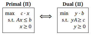
We can also write the dual linear program in exactly the same canonical form as the primal, by swapping the coefficient vector $ c $ and the objective vector $ b $, negating both vectors, and replacing the constraint matrix A with its negative transpose.

The Fundamental Theorem of Linear Programming. A linear program $\Pi$ has an optimal solution $x^{\star}$ if and only if the dual linear program $\amalg$ has an optimal solution $y^{\star}$ such that $ c x^{\star} = y^{\star} A x^{\star} = y^{\star} b $.

The weak form of this theorem is trivial to prove.

Weak Duality Theorem. If $ x $ is a feasible solution for a canonical linear program $\Pi$ and $ y $ is a feasible solution for its dual $\amalg$, then $ c x = y A x = y b $.

It immediately follows that if $ c x = y b $, then $ x $ and $ y $ are optimal solutions to their respective linear programs. This is in fact a fairly common way to prove that we have the optimal value for a linear program.

26.5 Duality Example

26.6 Strong Duality

The Fundamental Theorem can be rephrased in the following form:

Strong Duality Theorem. If $x^{\star}$ is an optimal solution for a canonical linear program $\Pi$, then there is an optimal solution $y^{\star}$ for its dual $\amalg$, such that $ c x^{\star} = y^{\star} A x^{\star} = y^{\star} b $.

证明略

26.7 Complementary Slackness

---

DAA - Chapter 3 - Rounding data and dynamic programming

Approximation algorithms can be designed using dynamic programming in a variety of ways, many of which involve rounding the input data in some way.

We can then show that by rounding the sizes of the large inputs so that, again, the number of distinct, large input values is polynomial in the input size and an error parameter, we can use dynamic programming to find an optimal solution on just the large inputs. Then this solution must be augmented to a solution for the whole input by dealing with the small inputs in some way.

DAA - Chapter 4 - Deterministic rounding of linear programs

---

Dealing with NP-hard Optimization Problems

An old engineering slogan says, “Fast. Cheap. Reliable. Choose two.”

Our goal so far in developing algorithms for optimization problems has been to find algorithms that

• $ (a) $ find the optimal solution;
• $ (b) $ run in polynomial time;
• $ (c) $ have property $ (a) $ and $ (b) $ for any input.

We have seen that we can indeed do this for optimization problems that can be formulated as a linear program. For problems that can be formulated as an integer linear program, we are not so lucky. In fact, unless P=NP, we cannot find algorithms that satisfy $ (a) $, $ (b) $ and $ (c) $ for a general integer linear program. Therefore, unless P=NP, we are going to have to focus on developing algorithms that have just two of the three properties (and do the best we can with respect to the other property).

In this lecture, we will illustrate these three approaches using vertex cover as an example.

Definition 1. Given an undirected graph $G = (V, E)$, the Minimum Vertex Cover (MVC) problem asks for a vertex cover of minimum size, i.e., a set of vertices $S \subseteq V$ of minimum size $\vert S \vert$ such that every edge $e \in E$ has at least one endpoint in $ S $.

The Minimum Vertex Cover problem is known to be NP-hard, so we don’t expect to find a polynomial time algorithm that finds the optimal solution for every possible input.

1. To drop requirement (c) $\Rightarrow$ Restricting Input (Structure)

If we drop requirement $ (c) $, and restrict our attention to certain classes of inputs, we can however have algorithms that solve the problem in polynomial time.

E.g. to restrict the input to bipartite graphs for Minimum Vertex Cover problem.

2. To drop requirement (b) $\Rightarrow$ Fixed Parameter Tractability (FPT)

Suppose we drop the requirement that we satisfy property $ (b) $, and we just try to find a minimum vertex cover with a “good” but not polynomial time algorithm.

Suppose that the size of the MVC is a fixed constant $k$, say $k = 2$ or $k = 3$ for some inputs. For such inputs, it is not hard to find a MVC in polynomial time.

• If we know the value $ k $, we just try all subsets of vertices of size $ k $, and check whether they are a vertex cover.
• There are $ n \choose k $ subsets of vertices of size $ k $, and checking each subset takes $ O(m) $ time, where $ n = \vert V \vert, m = \vert E \vert $.
• If we don’t know $ k $ in advance, we can find the MVC by checking whether there exists a vertex cover of size $l$ for $l = 0, l = 1, \dots , l = k$.
• Therefore, if the minimum vertex cover has size $ k $, we can find it in time $ O \left ( {n \choose 0} + {n \choose 1} + \dots + {n \choose k} \right ) \cdot O(m) = O(kn^km) $.

This is polynomial for fixed k, so for some inputs, this gives a polynomial time algorithm. However, this algorithm is far from practical (according to Kleinberg-Tardos, it will take longer than the age of the universe for an input with $n = 1000, k = 10$). Can we do something smarter?

Observation 1. If $ G $ has $ n $ vertices and a vertex cover of size $ k $, then $ G $ has at most $ k(n − 1) $ edges.

Proof. Each vertex can cover at most $ n − 1 $ edges, so $ k $ vertices can cover at most $ k(n − 1) $ edges. $\tag*{$\square$}$

Observation 2. Let $ e = \lbrace u, v \rbrace $ be any edge in $ G $. If $ G $ has a vertex cover of size $ k $, then either $ G \setminus \lbrace u \rbrace $ or $ G \setminus \lbrace v \rbrace $ has a vertex cover of size $ k − 1 $.

These two observations give rise to a simple recursive algorithm for finding a vertex cover of size $ k $ if it exists:

• If G has no edges, return the empty set.
• If G has more than $ k(\vert V \vert − 1) $ edges, then no vertex cover of size $ k $ exists.
• Else, let $ e = \lbrace u, v \rbrace $ be an edge of $ G $. – Find a vertex cover of size $ k − 1 $ in $ G \setminus \lbrace u \rbrace $ and in $ G \setminus \lbrace v \rbrace $.
  • If neither of those exists, then $ G $ has no vertex cover of size $ k $.
  • Else, if $ T $ is a vertex cover of size $ k − 1 $ of $ G \setminus \lbrace u \rbrace $ (respectively, $ G \setminus \lbrace v \rbrace $), then return $ T \cup \lbrace u \rbrace $ (respectively, $ T \cup \lbrace v \rbrace $).

Theorem 1. There exists an algorithm to check if a graph has a vertex cover of size $ k $ that runs in $ O(2^kn) $ time.

证明略

Note that this is pretty good: If $ k = O(\log n) $, then this is still a polynomial time algorithm. This is an example of a fixed parameter algorithm.

Definition 2. A problem is fixed parameter tractable (FPT) with respect to parameter $ k $ if there is an algorithm with running time at most $ f(k) n^{O(1)} $.

另参：Vertex Cover is Fixed-Parameter Tractable

3. To drop requirement (a) $\Rightarrow$ Approximation Algorithms

Another approach for dealing with NP-hardness is dropping the requirement $ (a) $ that the algorithm has to find the optimal solution. This is called a heuristic.

For the minimum vertex cover example, a reasonable heuristic seems to be the following:

• Repeat until $ E $ is empty
  • Pick a vertex $ v $ with highest degree,
  • Add $ v $ to $ S $, and remove $ v $ and its incident edges from $ G $.

Unfortunately, the solution returned by this heuristic can be pretty bad – there exists a family of examples for which the minimum vertex cover has size $ k! $ and the vertex cover found by the heuristic has size $ k! \log k $.

Definition 3. For a minimization problem, an $ \alpha $-approximation algorithm is an algorithm that runs in polynomial time and is guaranteed to output a solution of cost at most $ \alpha $ times the value of the optimal solution.

One popular approach to developing approximation algorithms is to use linear programming. We will see two exemplar algorithms:

• LP rounding
  1. Solve LP
  2. Then round to the ILP solution
• Primal-dual

3.1 LP rounding

We can formulate the MVC problem as an integer linear program (ILP) as follows. We slightly generalize the problem, and allow each vertex to have a nonnegative weight $ w_v \geq 0 $ that is part of the input. The problem in Definition 1 is then just the special case when $ w_v = 1 $ for all $ v \in V $.

For every vertex $ v \in V $ , we introduce a variable $ x_v \in \lbrace 0,1 \rbrace $. We think of $ x_v = 1 $ as representing that $ v \in S $. Then we want to minimize $ \sum_{v \in V} w_v x_v$, subject to the constraint that $ x_u + x_v \geq 1 $ for every $e = \lbrace u,v \rbrace \in E$. Let $OPT_{ILP}$ be the optimal value of this integer linear program (which is the same as the optimal value of the minimum vertex cover problem).

If we relax this integer program, we get the following LP:

\[\begin{align} \text{min } & \sum_{v \in V} w_v x_v \newline \text{s.t. } & x_u + x_v \geq 1 & \text{ for each } e = \lbrace u,v \rbrace \in E \newline & x_v \geq 0 & \text{ for } v \in V \tag{$P_{VC}$} \end{align}\]

(Note that we don’t need to require that $ x_v \leq 1 $, because this will automatically be true for any optimal solution!)

Theorem 2. There exists a $2$-approximation algorithm for the minimum vertex cover problem.

Proof. Let $ x^{\star} $ be an optimal solution to $P_{VC}$. Note that we can find $ x^{\star} $ in polynomial time. Also, now that $ \sum_{v \in V} w_v x_v^{\star} \leq OPT_{ILP} $, since the optimal integer solution gives a feasible solution to the LP with objective value $OPT_{ILP}$.

注意：

• $P_{VC}$ 是一个 LP 的问题
• $ x^{\star} $ 是$P_{VC}$ 的 optimal solution，即是 LP 的 optimal solution
• 但是 MVC 本身应该是一个 ILP 的问题
• 我们的目的是从 LP 的 solution 出发，rounding 到一个 ILP 的 solution
• 假设 MVC 的 ILP 的 optimal solution 是 $x’$，那么 $x’$ 一定是满足 $P_{VC}$ 的 LP 约束的，但不一定是 $P_{VC}$ 的最优解，所以 $ OPT_{ILP} = \sum_{v \in V} w_v {x_v}’ \geq \sum_{v \in V} w_v x_v^{\star} = OPT_{LP} $

Now, we just round up the variables $ x^{\star} $ that are greater than or equal to $\frac{1}{2}$. Let $x^{\dagger}$ be this rounded solution. Then $x_u^{\dagger} + x_v^{\dagger} \geq 1$ for every $\lbrace u,v \rbrace \in E$, since at least one of $ x_u^{\star} $ and $ x_v^{\star} $ must be at least $\frac{1}{2}$, so $x^{\dagger}$ is a feasible solution to vertex cover problem ($x^{\dagger}$ 确定会是一个 vertex cover，$x^{\star}$ 不一定是因为它不是整数 0 或者 1 的话就没有实际意义；但是，我们也无法保证 $x^{\dagger}$ 是 minimum 的). Also $\sum_{v \in V} w_v x_v^{\dagger} \leq 2 \sum_{v \in V} w_v x_v^{\star} \leq 2 OPT_{ILP}$. $\tag*{$\square$}$

Although this LP rounding algorithm is nice and seems simple, in some sense it is not that simple: it needs us to solve the LP relaxation, and–although we can do this in polynomial time–it is not “easy”. However, our knowledge of linear programming can also help us develop a very simple and fast algorithm.

3.2 Primal-dual algorithm

待续

---

Class

• 03/29/2016
  • Intro
  • Approx Alg
    • Example Problem: TSP / Metrix TSP
• 03/31/2016
  • Approx Alg
    • Continue with TSP / Metrix TSP
    • Shrink $\alpha < 2$
• 04/05/2016
  • PSS A
• 04/07/2016
  • Technique for Approx Alg (1): Linear Programming (LP)
    • Example Problem: Set Cover
    • Integer Linear Programming + Randomized Rounding
• 04/12/2016
  • Technique for Approx Alg (1): Linear Programming (LP)
    • Example Problem: Set Cover
    • Duality in Linear Programming / Dual Fitting
• 04/14/2016
  • Technique for Approx Alg (2): Semi-definite Programming (SDP)
    • Example Problem: Max Cut
    • Ellipsoid Method
• 04/19/2016
  • Technique for Approx Alg (2): Semi-definite Programming (SDP)
    • Continue with Max Cut
• 04/21/2016
  • Parameterized Complexity
    • Example Problem: Vertex Cover
    • Bounded Search Tree Method
    • Chorded Completion
• 04/26/2016
  • PSS B
• 04/28/2016
  • PSS B
• 05/03/2016
  • Fixed Parameter Tractability (FPT)
    • Example Problem: Vertex Cover
    • Kernelization Method
    • Crown Method

---

DAA - Chapter 5 - Random sampling and randomized rounding of linear programs

… Thus randomization gains us simplicity in our algorithm design and analysis, while derandomization ensures that the performance guarantee can be obtained deterministically.

5.1 Simple algorithms for MAX SAT and MAX CUT

In this section we will give a simple randomized $\frac{1}{2}$-approximation algorithm for each problem.

• MAX SAT
  • $n$ variables $x_1, \dots, x_n$
  • $m$ clauses $C_1, \dots, C_m$
    • In the form of $(x_p \vee \dots \vee x_q) \wedge (\dots)$
    • Every $x_i$ or $\overline{x_i}$ is a literal
      • $x_i$ is a positive literal
      • $\overline{x_i}$ is a negative literal
    • The number of literals in a clause is called its size or length.
      • The length of $C_j$ is $l_j$
    • Clauses of length 1 are sometimes called unit clauses
    • We assume that no literal is repeated in a clause and clauses are distinct
  • Nonnegative weight $w_j$ for each $C_j$
  • Objective: to find an assignment of TRUE/FALSE to the $x_i$s that maximizes the total weight of the satisfied clauses
    • A clause is satisfied if one of its $x_i$ is TRUE or $\overline{x_i}$ is FALSE

Theorem 5.1: Setting each $ x_i $ to TRUE with probability $\frac{1}{2}$ independently gives a randomized $\frac{1}{2}$-approximation algorithm for the MAX CUT problem.

Proof. Define a new random variable $ Y_j $ such that

\[\begin{align} Y_j = \left \lbrace \begin{matrix} & 1, & \text{if } C_j \text{ is satisfied} \newline & 0, & \text{otherwise} \end{matrix} \right. \end{align}\]

Total weights of the satisfied clauses $ W = \sum_{j=1}^m w_j Y_j $.

Then, by linearity of expectation and the definition of the expectation of a 0-1 random variable,

\[E[W] = \sum_{j=1}^{m} w_j E[Y_i] = \sum_{j=1}^{m} w_j \operatorname{Pr}[C_j \text{ is satisfied}]\]

Because $l_j \geq 1$,

\[\operatorname{Pr}[C_j \text{ is satisfied}] = 1 - \left ( \frac{1}{2} \right )^{l_j} \geq \frac{1}{2}\]

Hence,

\[E[W] = \sum_{j=1}^{m} w_j \cdot \frac{1}{2} = \frac{1}{2} \sum_{j=1}^{m} w_j \geq \frac{1}{2} OPT\]

$\tag*{$\square$}$

Observe that if $ l_j \geq k $ for each clause $ C_j $, then the analysis above shows that the algorithm is a $\big ( 1 - \left ( \frac{1}{2} \right )^k \big )$-approximation algorithm for such instances.

• MAX CUT
  • Undirected graph $G=(V,E)$
  • Nonnegative weight $w_{ij}$ for each edge $(i,j) \in E$
  • Cut $V$ into two partitions, $U$ and $W$
    • An edge across $U$ and $W$ is said to be “in the cut”
  • Objective: to find a cut to maximize the total weight of edges in the cut

Theorem 5.3: If we place each vertex $v$ into $U$ independently with probability $\frac{1}{2}$, then we obtain a randomized $\frac{1}{2}$-approximation algorithm for the MAX CUT problem.

Proof. Define a new random variable $ X_{ij} $ such that

\[\begin{align} X_{ij} = \left \lbrace \begin{matrix} & 1, & \text{if edge } (i,j) \text{ is in the cut} \newline & 0, & \text{otherwise} \end{matrix} \right. \end{align}\]

Total weights of the edges in the cut $ Z = \sum_{(i,j) \in E} w_{ij} X_{ij} $.

Then, by linearity of expectation and the definition of the expectation of a 0-1 random variable,

\[E[Z] = \sum_{(i,j) \in E} w_{ij} E[X_{ij}] = \sum_{(i,j) \in E} w_{ij} \operatorname{Pr}[\text{edge } (i,j) \text{ is in the cut}]\]

In this case, the probability that a specific edge $(i,j)$ is in the cut is easy to calculate: since the two endpoints are placed in the sets independently, they are in different sets with probability equal to $\frac{1}{2}$. Hence,

\[E[Z] = \sum_{(i,j) \in E} w_{ij} \cdot \frac{1}{2} = \frac{1}{2} \sum_{(i,j) \in E} w_{ij} \geq \frac{1}{2} OPT\]

$\tag*{$\square$}$

5.2 Derandomization

To derandomize a randomized algorithm means to obtain a deterministic algorithm whose solution value is as good as the expected value of the randomized algorithm.

Assume for the moment that we will make the choice of $x_1$ deterministically, and all other variables will be set true with probability $\frac{1}{2}$ as before.

略

It is sometimes called the method of conditional expectations, due to its use of conditional expectations.

略

5.3 Flipping biased coins

We will show here that biasing the probability with which we set $x_i$ is actually helpful; that is, we will set $x_i$ true with some probability not equal to $\frac{1}{2}$. To do this, it is easiest to start by considering only MAX SAT instances with no unit clauses $\overline{x_i}$, that is, no negated unit clauses. We will later show that we can remove this assumption.

Lemma 5.4: If each $x_i$ is set to true with probability $ p > \frac{1}{2} $ independently, then the probability that any given clause is satisfied is at least $ \min(p, 1−p^2) $ for MAX SAT instances with no negated unit clauses.

证明略

We can obtain the best performance guarantee by setting $ p = 1 − p^2 $. This yields $ p = \frac{1}{2} (\sqrt{5} − 1) \approx .618 $

略

5.4 Randomized rounding

The algorithm of the previous section shows that biasing the probability with which we set $x_i$ true yields an improved approximation algorithm. However, we gave each variable the same bias. In this section, we show that we can do still better by giving each variable its own bias. We do this by returning to the idea of randomized rounding.

we will create an integer program with a 0-1 variable $ y_i $ for each boolean variable $x_i$ such that $ y_i = 1 $ corresponds to $ x_i $ set true.

The integer program is relaxed to a linear program by replacing the constraints $ y_i \in \lbrace 0, 1 \rbrace $ with $ 0 \leq y_i \leq 1 $, and the linear programming relaxation is solved in polynomial time.

The central idea of randomized rounding is that the fractional value $ y_i^{\ast} $ is interpreted as the probability that $ y_i $ should be set to 1. In this case, we set each $ x_i $ to true with probability $ y_i^{\ast} $ independently.

We introduce a variable $ z_j $ for each clause $ C_j $ such that

\[\begin{align} z_j = \left \lbrace \begin{matrix} & 1, & \text{if } C_j \text{ is satisfied} \newline & 0, & \text{otherwise} \end{matrix} \right. \end{align}\]

For each clause $C_j$ let $P_j$ be the indices of the variables $x_i$ that occur positively in the clause, and let $N_j$ be the indices of the variables $x_i$ that are negated in the clause. We denote the clause $C_j$ by

\[\bigvee_{i \in P_j} x_i \vee \bigvee_{i \in N_j} \overline{x_i}\]

换句话说就是这样的：

• If $i \in P_j$, then positive literal $x_i$ is in $C_j$
• If $i \in N_j$, then negative literal $\overline{x_i}$ is in $C_j$

Then the inequality $\sum_{i \in P_j} y_i + \sum_{i \in N_j} (1-y_i) \geq z_j$ must hold for clause $C_j$.

• $\sum_{i \in P_j} y_i$ 即 $C_j$ 中 positive literal $x_i$ 取 TRUE 的个数
• $\sum_{i \in N_j} (1-y_i)$ 即 $C_j$ 中 negative literal $\overline{x_i}$ 取 FALSE 的个数

This inequality yields the following integer programming formulation of the MAX SAT problem:

\[\begin{align} \text{max } & \sum_{j=1}^m w_j z_j \newline \text{s.t. } & \sum_{i \in P_j} y_i + \sum_{i \in N_j} (1-y_i) \geq z_j, & \forall C_j = \bigvee_{i \in P_j} x_i \vee \bigvee_{i \in N_j} \overline{x_i} \newline & y_i \in \lbrace 0, 1 \rbrace, & i = 1,\dots,n, \newline & z_j \in \lbrace 0, 1 \rbrace, & j = 1,\dots,m. \end{align}\]

If $ Z_{ILP}^{\ast} $ is the optimal value of this integer program, then it is not hard to see that $ Z_{ILP}^{\ast} = OPT $.

The corresponding linear programming relaxation of this integer program is

\[\begin{align} \text{max } & \sum_{j=1}^m w_j z_j \newline \text{s.t. } & \sum_{i \in P_j} y_i + \sum_{i \in N_j} (1-y_i) \geq z_j, & \forall C_j = \bigvee_{i \in P_j} x_i \vee \bigvee_{i \in N_j} \overline{x_i} \newline & 0 \leq y_i \leq 1, & i = 1,\dots,n, \newline & 0 \leq z_j \leq 1, & j = 1,\dots,m. \end{align}\]

If $ Z_{LP}^{\ast} $ is the optimal value of this integer program, then clarly $ Z_{LP}^{\ast} \geq Z_{ILP}^{\ast} = OPT $.

待续

5.5 Choosing the better of two solutions

待续

5.6 Non-linear randomized rounding

In the case of the MAX SAT problem, we set $x_i$ to true with probability $ y_i^{\ast} $ . There is no reason, however, that we cannot use some function $ f:[0,1] \rightarrow [0,1] $ to set $x_i$ to true with probability $ f(y_i^{\ast}) $. Sometimes this yields approximation algorithms with better performance guarantees than using the identity function, as we will see in this section.

待续

DAA - Chapter 6 - Randomized rounding of semidefinite programs

So far we have used linear programming relaxations to design and analyze various approximation algorithms. In this section, we show how nonlinear programming relaxations can give us better algorithms than we know how to obtain via linear programming; in particular we use a type of nonlinear program called a semidefinite program. Part of the power of semidefinite programming is that semidefinite programs can be solved in polynomial time.

6.1 A brief introduction to semidefinite programming

Semidefinite programming uses symmetric, positive semidefinite matrices.

In what follows, vectors $ v \in \mathfrak{R}^n $ are assumed to be column vectors, so that $ v^T v $ is the inner product of $ v $ with itself, while $ vv^T $ is an $ n $ by $ n $ matrix.

Definition 6.1: A matrix $ X \in \mathfrak{R}^{n \times n} $ is positive semidefinite $ \iff \forall y \in \mathfrak{R}^n, y^TXy \geq 0 $.

Actually, $\forall y \in \mathfrak{R}^n$,

• $ y^TXy > 0 \iff X $ is positive definite
• $ y^TXy \geq 0 \iff X $ is positive semidefinite
• $ y^TXy < 0 \iff X $ is negative definite
• $ y^TXy \leq 0 \iff X $ is negative semidefinite

Sometimes we abbreviate “positive semidefinite” as “psd.” Sometimes we will write $X \succeq 0$ to denote that a matrix $X$ is positive semidefinite. Symmetric positive semidefinite matrices have some special properties which we list below. From here on, we will generally assume (unless otherwise stated) that any psd matrix $X$ is also symmetric.

Lemma: $C = \lbrace X \in \mathfrak{R}^{n \times n} \vert X \succeq 0 \rbrace$ is a convex region.

Proof: Equivalent to show that: given $X_1,X_2 \succeq 0$, $\forall t \in [0,1]$, we have $tX_1 + (1-t)X_2 \succeq 0$.

\[\begin{align} & \forall y, \quad y^TX_1y \geq 0, \quad y^TX_2y \geq 0 \newline \Rightarrow & \forall y, \quad t \cdot y^TX_1y \geq 0, \quad (1-t) \cdot y^TX_2y \geq 0 \newline \Rightarrow & \forall y, \quad y^T(tX_1)y \geq 0, \quad y^T \left ( (1-t)X_2 \right ) y \geq 0 \newline \Rightarrow & \forall y, \quad y^T \left ( tX_1 + (1-t)X_2 \right ) y \geq 0 \newline \Rightarrow & \left ( tX_1 + (1-t)X_2 \right ) y \succeq 0 \end{align}\]

$\tag*{$\square$}$

Fact 6.2: If $ X \in \mathfrak{R}^{n \times n} $ is a symmetric matrix, then the following statements are equivalent:

1. $X$ is psd
2. $X$ has eigenvalues $\geq 0$
   • If $\exists$ a vector $v \in \mathfrak{R}^n$ that $Xv = \lambda v$ for some scalar $\lambda$, then $\lambda$ is called the eigenvalue of $X$ with corresponding (right) eigenvector $v$
3. $X= V^T V$ for some $V \in \mathfrak{R}^{m \times n}$ where $m \leq n$
4. $X=\sum_{i=1}^n \lambda_i w_i w_i^T$ for some $\lambda_i \geq 0$ and vectors $ w_i \in \mathfrak{R}^n $ such that $w_i^T w_i = 1$ and $w_i^T w_j = 0$ for $i \neq j$

A semidefinite program (SDP) is similar to a linear program in that there is a linear objective function and linear constraints. In addition, however, a square symmetric matrix of variables can be constrained to be positive semidefinite. Below is an example in which the variables are $x_{ij}$ for $1 \leq i, j \leq n$.

\[\begin{align} \text{max or min } & \sum_{i,j} c_{ij} x_{ij} & \newline \text{subject to } & \sum_{i,j} a_{ijk} x_{ij} \leq b_k & \forall k \newline & x_{ij} = x_{ji} & \forall i,j \newline & X = (x_{ij}) \succeq 0 & \tag{6.1} \end{align}\]

We will often use semidefinite programming in the form of vector programming. The variables of vector programs are vectors $ v_i \in \mathfrak{R}^n $. We write the inner product of $v_i$ and $v_j$ as $v_i \cdot v_j$, or sometimes as $v_i^T v_j$.

\[\begin{align} \text{max or min } & \sum_{i,j} c_{ij} (v_i \cdot v_j) & \newline \text{subject to } & \sum_{i,j} a_{ijk} (v_i \cdot v_j) \leq b_k & \forall k \newline & v_i \in \mathfrak{R}^n & i=1,\dots,n \tag{6.2} \end{align}\]

We claim that in fact the SDP $(6.1)$ and the vector program $(6.2)$ are equivalent. This follows from Fact 6.2 Statement 3. Given a solution to the SDP, we can take the solution $X$, compute in polynomial time a matrix $V$ for which $X = V^T V$ and set $v_i$ to be the $i^{th}$ column of $V$.

6.2 MAX CUT + SDP

Recall that for this problem, the input is an undirected graph $G = (V,E)$, and nonnegative weights $w_{ij} \geq 0$ for each edge $(i, j) \in E$. The goal is to partition the vertex set into two parts, $U$ and $W$ so as to maximize the total weight of the edges in the cut.

For every vertex $v_i$, define

\[\begin{align} y_i = \left \lbrace \begin{matrix} & -1, & \text{if } v_i \in U \newline & +1, & \text{if } v_i \in W \end{matrix} \right. \end{align}\]

Note that if an edge $(i, j)$ is in this cut, then $y_i y_j = −1$, while if the edge is not in the cut, $y_i y_j = 1$. Then MAX CUT can be modeled as

\[\begin{align} \text{maximize } & \frac{1}{2} \sum_{(i,j) \in E} w_{ij} (1 - y_i y_j) & \newline \text{subject to } & y_i \in \lbrace -1, +1 \rbrace & i=1,\dots,n \tag{$CUT_{max}$} \end{align}\]

We can now consider the following vector programming relaxation of $CUT_{max}$

\[\begin{align} \text{maximize } & \frac{1}{2} \sum_{(i,j) \in E} w_{ij} (1 - v_i \cdot v_j) & \newline \text{subject to } & v_i \cdot v_i = 1 & i=1,\dots,n \newline & v_i \in \mathfrak{R}^n & i=1,\dots,n \tag{6.4} \end{align}\]

$(6.4)$ is a relaxation of $CUT_{max}$ since we can take any feasible solution $y$ of $CUT_{max}$ and produce a feasible solution to $(6.4)$ of the same value by setting $v_i = (y_i, 0, 0, \dots, 0)$: clearly $v_i \cdot v_i = 1$ and $v_i \cdot v_j = y_i y_j = 1$. Thus if $Z_{VP}$ is the value of an optimal solution to the vector program, it must be the case that $Z_{VP} \geq OPT_{CUT}$.

We can solve $(6.4)$ in polynomial time. We would now like to round the solution to obtain a near-optimal cut. To do this, we introduce a form of randomized rounding suitable for vector programming.

注：这和前面 ILP 的套路是一样的：

\[\text{problem} \rightarrow ILP \overset{\text{relax}}{\rightarrow} LP \rightarrow LP \text{ solution} \overset{\text{round}}{\rightarrow} ILP \text{ solution}\] \[\text{problem} \rightarrow IQP \overset{\text{relax}}{\rightarrow} QP \rightarrow QP \text{ solution} \overset{\text{round}}{\rightarrow} IQP \text{ solution}\]

$QP$ for Quadratic Programming; $IQP$ for Integer Quadratic Programming。而 $SDP / VP$ 正是 $QP$ 的 special case。

我们同样可以用 randomized rounding 来处理 $Z_{VP}$。而这个 randomized rounding 的处理过程又能看成 “choosing a random hyperplane”。因为 $v_i$ 都是 unit vector，所以所有的 $v_i$ 都在一个 unit sphere 上。rounding 的过程就好比把这个 unit sphere 用一个 hyperplane 一刀切，一个 half-space 算 $U$，另一个 half-space 算 $W$ (联想 LP 的 $y_i$ 按 0.5 一刀切，大于的算 1，小于的算 0)。假设 $v_i$ 和 $v_j$ 的夹角是 $\theta$，一个 random 的 hyperplane 能正好把 $v_i$ 和 $v_j$ 切开的概率是 $\frac{\theta}{\pi}$。

又因为 $v_i \cdot v_j = \lvert v_i \rvert \lvert v_j \rvert \cos \theta = \cos \theta$，所以 $\theta = \arccos(v_i \cdot v_j)$。

又因为 $\frac{\theta}{\pi} = \frac{\arccos(v_i \cdot v_j)}{\pi} \geq 0.878 \cdot \frac{1}{2} (1 - v_i \cdot v_j)$，所以 rounding 得到的 solution $\geq 0.878 \cdot Z_{VP} \geq 0.878 \cdot OPT_{CUT}$.

待续：Ellipsoid Method + Separation Oracle

6.3 Approximating QP

6.4 Finding a correlation clustering

6.5 Coloring 3-colorable graphs

---

Fixed Parameter Algorithms: Part 1

Classical complexity

• We usually aim for poly-time algorithms: $O(n^c)$
• It is unlikely that poly-time algorithms exist for NP-hard problems.
• We expect that these NP-hard problems can be solved only in exponential time: $O(c^n)$

Parameterized complexity

Instead of expressing the running time as a function $T(n)$ of $n$, we express it as a function $T(n, k)$ of the input size $n$ and some parameter $k$ of the input.

The existence of efficient, exact, and deterministic solving algorithms for NP-complete, or otherwise NP-hard, problems is considered unlikely, if input parameters $k$ are not fixed; all known solving algorithms for these problems require time that is exponential (or at least superpolynomial) in the total size of the input, $n$.

However, some problems can be solved by algorithms that are exponential only in the size of a fixed parameter $k$ while polynomial in the size of the input $n$.

• Hence, if k is fixed at a small value and the growth of the function over k is relatively small then such problems can still be considered “tractable” despite their traditional classification as “intractable”.
  • Such an algorithm is called a fixed-parameter tractable (fpt-)algorithm
  • Problems in which some parameter $k$ is fixed are called parameterized problems.
  • A parameterized problem that allows for such an fpt-algorithm is said to be a fixed-parameter tractable problem and belongs to the complexity class $FPT$.

To be specific,

• A parameterized problem is a language $L \subseteq \Sigma^{\ast} \times \mathbb{N}$, where $\Sigma$ is a finite alphabet.
  • The second component is called the parameter of the problem.
• A parameterized problem $L$ is fixed-parameter tractable if the question “$(x, k) \in L$?” can be decided in running time $f(k) \cdot \lvert x \rvert^{O(1)}$, where $f$ is an arbitrary function depending only on $k$.
  • The corresponding complexity class is called $FPT$.

For example, there is an algorithm which solves the vertex cover problem in $O(kn + 1.274^k)$ time. This means that vertex cover is fixed-parameter tractable with the size of the solution as the parameter.

For $FTP$:

• Typically, the function $f(k)$ is thought of as single exponential, such as $2^{O(k)}$ but the definition admits functions that grow even faster.
• The crucial part of the definition is to exclude functions of the form $f(n,k)$, such as $n^k$.
• The class $FPL$ (fixed parameter linear) is the class of problems solvable in time $f(k) \cdot \lvert x \rvert$.
  • $FPL$ is thus a subclass of $FPT$.
• There are a number of alternative definitions of $FPT$.
  • E.g., the running time requirement can be replaced by $f(k) + \lvert x \rvert^{O(1)}$.
  • Also, a parameterised problem is in $FPT$ if it has a so-called kernel. Kernelization is a preprocessing technique that reduces the original instance to its “hard kernel”, a possibly much smaller instance that is equivalent to the original instance but has a size that is bounded by a function in the parameter.
• $FPT$ is closed under a parameterised reduction called fpt-reduction.
• Obviously, $FPT$ contains all polynomial-time computable problems.

Powerful toolbox for designing FPT algorithms

• Bounded Search Tree
• Graph Minors Theorem
• Color coding
• Kernelization
• Treewidth
• Iterative compression

$O^{\ast}$ notation: $O^{\ast}(f(k))$ means $O(f(k) \cdot n^c)$ for some constant $c$.

Kernelization

In parameterized complexity theory, it is often possible to prove that a kernel with guaranteed bounds on the size of a kernel (as a function of some parameter associated to the problem) can be found in polynomial time. When this is possible, it results in a fpt-algorithm whose running time is the sum of the (polynomial time) kernelization step and the (non-polynomial but bounded by the parameter) time to solve the kernel. Indeed, every problem that can be solved by a fixed-parameter tractable algorithm can be solved by a kernelization algorithm of this type.

Definition: P23

Kernelization for VERTEX COVER: P26,27,29,32-35

COVERING POINTS WITH LINES: P38

Some kernelizations are based on surprising nice tricks (E.g. Crown Reduction and the Sunflower Lemma).

Crown Reduction: P43,45,46,47,48,49,50. Proof of Lemma.

DUAL OF VERTEX COLORING: P54,55

Sunflower lemma: P57,58,59

Bounded search tree method

P61-72

待续

Fixed Parameter Algorithms: Part 2

The Party Problem (MWIS)

• Problem: Invite some colleagues for a party.
• Maximize: The total fun factor of the invited people.
• Constraint:
  • Everyone has a fun positive factor.
  • Do not invite a colleague and his direct boss at the same time!

Actually a Maximum-Weight Independent Set (MWIS) problem.

In graph theory, an independent set or stable set is a set of vertices in a graph, no two of which are adjacent.

That is, for every two vertices in independent set $S$, there is no edge connecting them.

• Fan factors are weights.
• MWIS in a tree (not a general graph) in this case.
  • Boss-colleague => root-leaf hierarchy

Solve by DP.

• $T_v$: the subtree rooted at node $v$
• $A[v]$: max weight of an independent set of $T_v$
• $B[v]$: max weight of an independent set of $T_v \setminus \lbrace v \rbrace$

Goal: $A[r]$ for root $r$

Method: Assume $v_1, \dots, v_k$ are children of $v$. Use the recurrence

\[\begin{align} B[v] = \sum_{i=1}^{k} A[v_i] \newline A[v] = \max \lbrace B[v], w(v) + \sum_{i=1}^{k}B[v_i] \end{align}\]

The values $A[v]$ and $B[v]$ can be calculated in a bottom-up order (the leaves are trivial).

Treewidth

A measure of how “tree-like” the graph is.

A tree decomposition (wikipedia) of a graph $G = (V, E)$ is a tree, $T$, with nodes $X_1, \dots, X_n$, where each $X_i$ is a subset of $V$, satisfying the following properties:

1. For each vertex $v \in V$, there is at least one tree node $X_i$ that contains $v$ (denoted by $v \in X_i$).
   • Therefore, $\bigcup_{i=1}^n X_i = V$.
2. If both $X_i$ and $X_j$ contain $v$, then all $X_k$ in the (unique) $X_i \rightsquigarrow X_j$ path in $T$ also contains $v$.
   • Why unique? Because it is a tree property that any two vertices in a tree can be connected by a unique simple path.
   • Equivalently, all $X_i$s containing a certain vertex $v$ form a connected subtree of $T$.
     • By definition, a path is definitely a tree.
3. For each edge $(u,v) \in E$, there is at least one tree node $X_i$ that contains both $u$ and $v$.
   • Suppose:
     • $\exists X_i$ such that $u \in X_i$ and $v \in X_i$
     • All nodes containing $u$ form a subtree $T’_u$
     • All nodes containing $v$ form a subtree $T’_v$
   • Then $X_i \in T’_u$, $X_i \in T’_v$ and thus $X_i \in T’_u \cap T’_v$.

The width of a tree decomposition is $width(T)=\max_i \lvert X_i \rvert - 1$. A graph can have different tree decompositions $T_1,\dots,T_m$, so the treewidth of $G$ is $tw(G) = \min_j width(T_j)$.

Special cases:

• $tw(T)=1$ for any tree $T$
  • Actually, $tw(G)=1 \iff G \text{ is a forest}$
• $tw(H) \leq 3$ for any Halin graph $H$
• $tw(C_n) = 2$ for any cycle
• $tw(K_n) = n-1$ for any complete graph
• $tw(K_{(m,n)}) = \min(m,n)$ for any complete bipartite graph
• $tw(P_m \square P_n) = min(m,n)$ where $P_m \square P_n$ is an $m \times n$ grid

Finding tree decompositions

P19

Algoritmhs for bounded-treewidth graphs

MWIS: P21-25

3-COLORING: P26-29

Hamiltonian cycle: P30-49

Monadic Second Order Logic: P51

Courcelle’s Theorem: P52-57

SUBGRAPH ISOMORPHISM: P58-60

Graph-theoretical properties of treewidth

Applications

Baker’s shifting strategy: delete the $L_i$ layer. P87

PTAS: P100

待续

---

Treewidth @ Erickson §11

11.1 Definitions

Revised definition: A graph $G$ is called a $k$-tree if and only if

• either $G = K_k$ (complete graph with $k$ vertices),
  • – OR –
• $G$ has a vertex $v$ with degree $k$ such that such that the (open) neighborhood of $v$ forms a $k$-clique, and $G \setminus \lbrace v \rbrace$ is a $k$-tree.

The bottom-up definition:

• $K_k$ is a $k$-tree.
• A $k$-tree $G$ with $n+1$ vertices ($n \geq k$) can be constructed from a $k$-tree $H$ with $n$ vertices by adding a vertex adjacent to exactly $k$ vertices that form a $k$-clique in $H$.
  • From LINEAR TIME ALGORITHMS FOR NP-HARD PROBLEMS RESTRICTED TO PARTIAL $k$-TREE: One can test a graph for being a $k$-tree by repeatedly removing a vertex of degree $k$ with completely connected neighbors (a $k$-leaf) until no such vertex remains, then the graph is a $k$-tree if and only if what remains is $K_k$
• No other graphs are $k$-trees.

Observation: a connected graph $G$ is a $1$-tree $\iff$ $G$ is a tree.

注意： $K_2$ 是一棵树，然后也是一棵 $2$-tree；但同时也是一棵 $1$-tree。也就是说 “$G$ is a $2$-tree” 的同时也可以有 “$G$ is a $1$-tree”；这两句陈述并不存在排斥或冲突的情形。

A partial $k$-tree is any subgraph of a $k$-tree.

• For any fixed constant $k$, a graph $G$ with $tw(G) \leq k$ is called a partial $k$-tree.

Lemma 11.1 A graph has treewidth $k$ if and only if it is a partial $k$-tree.

• 结合上一条，如果 $tw(G) = j < k$，首先 $G$ 一定是一个 partial $j$-tree，同时 $G$ 也是一个 partial $k$-tree (just image $G$ as a subtree of a $k$-tree)

---

PTAS & Distance in Graphs & Baker’s technique

PTAS: Polynomial-Time Approximation Scheme

• A PTAS is an algorithm which takes an instance of an optimization problem $L$ and a parameter $\epsilon > 0$ and, in polynomial time, produces a $(1+\epsilon)$-approximation (or $(1-\epsilon)$ for maximization problems) alg for $L$.
• The running time of a PTAS is required to be polynomial in $n$ for every fixed $\epsilon$ but can be different for different $\epsilon$. E.g.
  • $n^{O(\frac{1}{\epsilon})}$
  • $2^{O(\frac{1}{\epsilon})} n^2$: a.k.a. EPTAS (efficient PTAS)
  • $O(\frac{1}{\epsilon^2} n)$: a.k.a. FPTAS (full PTAS)

Let $G$ be an undirected graph: (参考 Diameter vs Radius in Maximal Planar Graphs)

• The eccentricity of a vertex $v$ of $G$, is the maximum distance between $v$ and any other vertex of $G$: $ecc(v)=\max_udist(v,u)$.
• The radius of $G$ is the minimum eccentricity among all vertices in $G$:$R(G)=\min_v ecc(v)$.
  • A spanning tree of a graph $G$ is a subgraph that is a tree and contains every vertex of $G$.
  • $R(G) = r \Rightarrow G$ has a rooted spanning tree of height $r$
  • A disconnected graph therefore has infinite radius.
• The diameter of $G$ is the maximum eccentricity among all vertices in $G$: $G$:$D(G)=\max_v ecc(v)$.
  • $R(G) \leq D(G) \leq 2R(G)$

Lemma: $\forall$ planar graph $G$ with $R(G) = r$, $tw(G) \leq 3r$.

Apply Baker’s technique to MWIS in a planar graph

An independent set of a graph $G$ is a set of vertices in $G$, no two of which are adjacent. In Maximum Weighted Independent Set (MWIS) problem, each vertex is assigned a weight.

Let $G$ be a planar graph. Choose an arbitrary vertex $r$ as root and build a spanning tree via BFS.