Smoothing
总结自 2. Smoothing。
In the context of nonparametric regression, a smoothing algorithm (a.k.a. a smoother) is a summary of trend in $Y$ as a function of explanatory variables $X_1, \dots, X_p$. The smoother takes data and returns a function, called a smooth.
We focus on scatterplot smooths, for which $p = 1$.
Essentially, a smooth just finds an estimate of $f$ in the nonparametric regression function $Y = f(x) + \epsilon$.
As a running example for the next several sections, assume we have data generated from the following function by adding $\mathcal{N}(0,.25)$ noise.
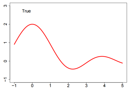

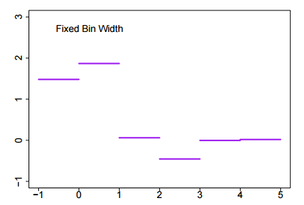
1. Bin Smoothing
Partition $\mathbb{R}^p$ into disjoint bins. For $p = 1$ take $\lbrace [i, i + 1), i \in \mathbb{Z} \rbrace$. Within each bin average the $Y$ values to obtain a smooth that is a step function.
2. Moving Averages
Moving averages use variable bins containing a fixed number of observations, rather than fixed-width bins with a variable number of observations. They tend to wiggle near the center of the data, but flatten out near the boundary of the data.

3. Running Line
This improves on the moving average by fitting a line rather than an average to the data within a variable-width bin. But it still tends to be rough.

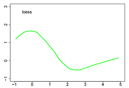
4. Loess
Loess extends the running line smooth by using weighted linear regression inside the variable-width bins. Loess is more computationally intensive, but is often satisfactorily smooth and flexible.
LOESS fits the model
\[\mathrm{E}(Y) = \theta(x)^{T} x\]where
\[\hat{\theta}(x) = \underset{\theta \in \mathbb{R}^p}{\operatorname{argmin}} \sum_{i=1}^{n} w(\lVert x - X_i \rVert)(Y_i - \theta^T X_i)^2\]and $w$ is a weight function that governs the influence of the $i^{\text{th}}$ datum according to the (possibly Mahalanobis) distance of $X_i$ from $x$.
LOESS is a consistent estimator, but may be inefficient at finding relatively simple structures in the data. Although not originally intended for high-dimensional regression, LOESS is often used.
5. Kernel Smoothers
These are much like moving averages except that the average is weighted and the bin-width is fixed. Kernel smoothers work well and are mathematically tractable. The weights in the average depend upon the kernel $K(x)$. A kernel is usually symmetric, continuous, nonnegative, and integrates to 1 (e.g., a Gaussian kernel).
The bin-width is set by $h$, also called the bandwidth. This can vary, adapting to information in the data on the roughness of the function.
Let $\lbrace (y_i, x_i) \rbrace$ denote the sample. Set $K_h(x) = h^{-1}K(h^{-1}x)$. Then the Nadaraya-Watson estimate of $f$ at $x$ is
\[\hat{f}(x) = \frac{\sum_{i=1}^{n} K_h(x - x_i)y_i}{\sum_{i=1}^{n} K_h(x - x_i)}\]For kernel estimation, the Epanechnikov function has good properties. The function is
\[K(x) = {3 \over 4}(1 - x^2), -1 \leq x \leq 1\]6. Splines
If one estimates $f$ by minimizing the equation that balances least squares fit with a roughness penalty, e.g.,
\[\underset{f \in \mathcal{F}}{\min} \sum_{i=1}^{n} \left [ y_i - f(x_i) \right ]^2 + \lambda \int \left [ f^{(k)}(x) \right ]^2 dx\]over an appropriate set of functions (e.g., the usual Hilbert space of square-integrable functions), then the solution one obtains are smoothing splines.
Smoothing splines are piecewise polynomials, and the pieces are divided at the sample values $x_i$.
The $x$ values that divide the fit into polynomial portions are called knots. Usually splines are constrained to be smooth across the knots.
Regression splines have fixed knots that need not depend upon the data. But knot selection techniques enable one to find good knots automatically.
Splines are computationally fast, enjoy strong theory, work well, and are widely used.

7. Comparing Smoothers
Most smoothing methods are approximately kernel smoothers, with parameters that correspond to the kernel $K(x)$ and the bandwidth $h$.
In practice, one can:
- fix $h$ by judgment
- find the optimal fixed $h$
- fit $h$ adaptively from the data
- fit the kernel $K(x)$ adaptively from the data
There is a point of diminishing returns, and this is usually hit when one fits the h adaptively.
Silverman (1986; Density Estimation for Statistics and Data Analysis, Chapman-Hall) provides a nice discussion of smoothing issues in the context of density estimation.
Breiman and Peters (1992; International Statistics Review, 60, 271-290) give results on a simulation experiment to compare smoothers. Broadly, they found that:
- adaptive kernel smoothing is good but slow,
- smoothing splines are accurate but too rough in large samples,
- everything else is not really competitive in hard problems.
Theoretical understanding of the properties of smoothing depends upon the eigenstructure of the smoothing matrix. Hastie, Tibshirani, and Freidman (2001; The Elements of Statistical Learning, Springer) provide an introduction and summary of this area in Chapter 5.
A key issue is the tension between how “wiggly” (扭曲的;与 “平滑” 对应) (or flexible) the smooth can be, and how many observations one has. You need a lot of data to fit local wiggles. This tradeoff is reflected in the degrees of freedom associated with the smooth.
In linear regression one starts with a quantity of information equal to $n$ degrees of freedom where $n$ is the number of independent observations in the sample. Each estimated parameter reduces the information by 1 degree of freedom. This occurs because each estimate corresponds to a linear constraint in $\mathbb{R}^n$, the space in which the $n$ observations lie.
Smoothing is a nonlinear constraint and costs more information. But most smoothers can be expressed as a linear operator (matrix) $S$ acting on the response vector $y \in \mathbb{R}^n$. It turns out that the degrees of freedom lost to smoothing is then $tr(S)$.
In linear regression, the “smoother” is the linear operator that acts on the data to produce the estimate:
\[\hat{y} = SY = X(X^T X)^{-1} X^T Y\]The matrix $S$ is sometimes called the hat matrix.
Note that:
\[\begin{align} tr[S] &= tr[X(X^T X)^{-1} X^T Y] \newline &= tr[X^T X (X^T X)^{-1}] \newline &= tr[I] \newline &= p \end{align}\]since $X$ is $n \times p$ and from matrix algebra we know that $tr[ABC] = tr[CAB]$ (see Graybill, Applied Matrix Algebra in the Statistical Sciences, 1983, for a proof).
This means that the degrees of freedom associated fitting a linear regression (without an intercept) is $p$. Thus one has used up an amount of information equivalent to a random sample of size $p$ in fitting the line, leaving an amount of information equivalent to a sample of size $n − p$ with which to estimate dispersion or assess lack of fit.
If one uses an intercept, then this is equivalent to adding a column of ones to $X$, so its dimension is $n \times (p + 1)$ and everything sorts out as usual.
Similarly, we can find the smoothing operator for bin smoothing in $\mathbb{R}^1$. Here one divides a line segment $(a, b)$ into $m$ equally spaced bins, say $B_1, B_2, \dots, B_m$. Assume there are $k_j$ observations whose $x$-values lie in $B_j$. Then the bin estimate is:
\[\hat{y} = SY = {1 \over k_j}\sum_{i=1}^{n} Y_i I_{B_j}(X_i)\]In this case the matrix $S$ is a block matrix whose diagonal blocks are $k_j \times k_j$ submatrices whose every entry is $1 \over k_j$, and the off-diagonal blocks are matrices of zeroes.
Clearly, the trace of this matrix is $m$, since the diagonal of each block adds to 1.
Most smoothers are shrinkage estimators. Mathematically, they pull the weights on the coefficients in the basis expansion for $y$ towards zero.
Shrinkage is why smoothing has an effective degrees of freedom between $p$ (as in regression, which does not shrink) and $n$ (which is what one would expect from a naive count of the number of parameters needed to make the function perfectly fit each data point).
For bin smoothing we can oversmooth or undersmooth. If $m \ll n$, there are few bins and the fitted function has very few jumps (and so is oversmoothed). But if $m$ is large (say equal to $n$ with the bins chosen so that each contains exactly one observation), then the degrees of freedom is $n$ and one has undersmoothed.
Smoothing entails a tradeoff between the bias and variance in $\hat{f}$. If one undersmooths, $\hat{f}$ is wiggly (high variance) but has low bias. If one smooths too much, $\hat{f}$ has small variance but high bias.
Mean squared error is a criterion that captures both aspects. At $x$,
\[MSE[\hat{f}] = \mathrm{E}[(\hat{f}(x)−f(x))^2] = \mathrm{Var}[\hat{f}(x)] + \mathrm{bias}^2[\hat{f}(x)].\]One wants a smooth that minimizes $MSE[\hat{f}]$ over all $x$.
待补充:
http://www.biostat.jhsph.edu/~ririzarr/Teaching/754/ https://web.stanford.edu/~hastie/Papers/lsam_annals.pdf http://www.stat.umn.edu/geyer/5601/notes/smoo.pdf http://www.stat.uchicago.edu/~lafferty/pdf/nonparam.pdf http://data.princeton.edu/eco572/smoothing.pdf
Comments