Digest of Essence of Linear Algebra
Greatest thanks to 3Blue1Brown!
Chapter 1 - Vectors, what even are they?
The introduction of numbers as coordinates (by reference to the the particular division scheme of the open one-dimensional continuum) is an act of violence. ―Hermann Weyl
Mathematicians’ perspective:
- A vector can be anything where there’s a sensible notion of adding two vectors and multiplying a vector by a number.
- I.e. 只要实现了 “可以两两相加” 和 “可以与一个数相乘” 的都可以叫 vector
- Linear algebra revolves around vector addition and scalar multiplication. 线性代数是紧紧围绕着这两个基本概念的。
如果要从 geometrics 的角度来理解的话,我们最好把每个 vector 都理解为:
- An arrow inside a coordinate system, with it’s tail sitting at the origin (原点) (Sorry, Hermann Weyl)
- 虽然理论上,vectors can freely sit anywhere in the space.
- A vector $\vec v = \icol{a \newline b}$ gives instructions for how to get from its tail to its tip.
- First walk along 1st axis for $a$ units;
- then walk along 2nd axis for $b$ units.
1.1 Adding two vectors
假设有 $\vec v = \icol{a \newline b}$ 和 $\vec w = \icol{c \newline d}$,那么 vector 加法 $ \vec v + \vec w$ 可以理解为:
- First walk along 1st axis for $a$ units;
- then walk along 2nd axis for $b$ units;
- then walk along 1st axis for $c$ units;
- then walk along 2nd axis for $d$ units.
- 或者
- First walk along 1st axis for $a+c$ units;
- then walk along 2nd axis for $b+d$ units.
- 简单的实数加法也可以这么理解,比如 $2+5$:
- First walk (along the only axis) for $2$ units;
- then walk for $5$ units;
- you would walk $7$ units in total.
1.2 Multiplying a vector by a number
- $2 \cdot \vec v$ means you stretch out $\vec v$ so that it’s $2$ times as long as before.
- First walk along 1st axis for $2a$ units;
- then walk along 2nd axis for $2b$ units.
- $-2 \cdot \vec v$ means first flip $\vec v$ then stretch it out by factor of $2$.
- $\frac{1}{3} \cdot \vec v$ means you squash it down so that it’s $\frac{1}{3}$ of the original length.
This process of 1) stretching or 2) squashing or 3) sometimes reversing the direction of a vector is called scaling. The number you used to scale the vector is called a scalar. (翻译为 “标量”. Never mind.) In fact, throughout linear algebra, one of main things that numbers do is to scale vectors.
Chapter 2 - Linear combinations, span, and basis vectors
Mathematics requires a small dose, not of genius, but of imaginative freedom which, in a larger dose, would be insanity. ―Angus K. Rodgers
Unit vector: a vector that has a magnitude of one.
- Unit vector in $x$-direction $\hat i = \icol{1 \newline 0}$
- Unit vector in $y$-direction $\hat j = \icol{0 \newline 1}$
Think about each coordinate in $\icol{a \newline b}$ as a scalar. Then $\vec v = \icol{a \newline b} = a \hat i + b \hat j$. In this sense, $\icol{a \newline b}$ describes $\vec v$ as the sum of two scaled vectors. This is a surprisingly importance concept in linear algebra.
- Together, $\hat i$ and $\hat j$ are called the basis vectors of a $xy$ coordinate system. (坐标系的基向量)
- When you think about coordinates in $\vec v$ as scalars, the basis vectors are what those scalars scale to represent $\vec v$
What if we chose some arbitrary vectors as basis vectors? We could have done so and gotten a completely reasonable, new coordinate system.
- 亦即,如果有 $\vec v = a \vec p + b \vec q$,我们可以想象有一个 “$pq$ coordinate system”,它以 $\vec p$ 和 $\vec q$ 为 basis vectors,那么 $\vec v = a \vec p + b \vec q$ 就相当于是这个 $pq$ coordinate system 的一个 arrow 指向 $(a,b)$ 这个点。
Suppose $\vec p$ and $\vec q$ are 2-D vectors. Choose any possible $a$ and $b$ for $\vec v = a \vec p + b \vec q$. How many $\vec v$ can you get? The answer is that you can get every possible 2-D vectors. This means that a pair of 2-D basis vectors gives us a valid way to go back and forth between pairs of numbers and 2-D vectors.
- Rule of thumb: any time we describe vectors numerically, it depends on an implicit choice of what basis vectors we’re using.
Any time you scale two vectors and adding them like this, it’s called a linear combination of those two vectors.
- You can see “linear” this way: if you fix one scalar and let the other one change its value freely, the tips of the resulting vectors would draw a straight line.
- When your original vectors happen to line up (共线),the tip of the resulting vector is limited to exactly the same line.
- If both vectors are zero, you’d just be stuck at the origin.
The span of $\vec p$ and $\vec q$ is the set of all possible vectors you can reach with a linear combination of them, or put simply is the set of all their linear combinations. So restating what we just discussed,
- The span of most 2-D vectors is all vectors in this 2-D space.
- When they line up, their span is all vectors whose tips sit on that line.
- The span of two vectors is basically a way of asking what are all the possible vector you can reach using only the 2 fundamental operations of vectors–vector addition and scalar multiplication.
Vectors vs Points
In general, if you’re thinking about a vector on its own, think of it as an arrow. And if you’re dealing with a collections of vectors, it’s convenient to think of them all as points.
- The span of most 2-D vectors ends up being the entire infinite sheet of the 2-D space.
- When they line up (共线), their span is just that line.
In 3-D cases:
- Take 2 vectors in 3-D space that point in different directions. Their span is a flat sheet cutting through the origin of the 3-D space.
- Take 3 vectors:
- If the 3rd vector happens to be sitting on the span of the first two, their span would still be the flat sheet.
- In other words, adding a scaled 3rd vector to the linear combination doesn’t really give you access to any new vectors.
- Otherwise the span would be the whole of the 3-D space.
- You can imagine this way: when you scale the 3rd vector, it moves the span of the first 2 vectors along its direction, sweeping the flat sheet through all the 3-D space.
- If the 3rd vector happens to be sitting on the span of the first two, their span would still be the flat sheet.
In the case where the 3rd vector was already sitting on the span of the first two, or the case where two vectors happen to line up, at least one of these vectors is redundant, not adding anything to our span. Whenever this happens, you could remove one vector without reducing then span. We say that these vectors are linearly dependent.
- Another way of phrasing that would be to say that one of the vectors can be expressed as a linear combinations of the others, since it’s already in the span of the others.
On the other hand, if each vector really add another dimension to the span, they are said to be linearly independent.
\[\vec u \text{ is linearly independent to } \vec v, \vec w \iff \forall a \text{ and } b, \vec u \neq a \vec v + b \vec w\]Technical definition of basis:
- The basis of a vector space is a set of linearly independent vectors that span this full space.
- $\hat i$ and $\hat j$ are called the basis vectors
- 它们俩合起来称作(被它们 span 构成的)2-D space 的 basis
Chapter 3 - Linear transformations and matrices
Unfortunately, no one can be told what The Matrix is. You have to see it for yourself. ―Morpheus
Transformation is essentially a fancy word for “function”. 把 $xy$ 坐标画成网格,线性变换会旋转、拉伸、翻转这个网格(比如从正方形的格子变成菱形的)
Visually speaking, a transformation is linear if it has two properties:
- all lines (平面内的所有 lines,不单单只是网格线) must remain lines, without getting curved;
- and the origin must remain fixed in place
(满足 1 但是不满足 2 的我们称为 Affine Transformation,仿射变换)
In general, you should think of linear transformations as “keeping grid lines parallel and evenly spaced” (保持网格线平行并等距分布).
How would you describe one of these numerically? What formula did you give to the comupter so that if you give it the coordinates of a vector, it can give you the coordinates of where that vector lands (in the transformed space)? It turns out that you only need to record where the two basis vectors, $\hat i$ and $\hat j$, each land.
E.g. $\vec v = x \hat i + y \hat j \Rightarrow \text{Transformed } \vec v = x (\text{Transformed } \hat i) + y (\text{Transformed } \hat j)$
$\vec v = \icol{x \newline y} = x \icol{1 \newline 0} + y \icol{0 \newline 1} \Rightarrow \text{Transformed } \vec v = x \icol{i_1 \newline i_2} + y \icol{j_1 \newline j_2} = \icol{i_1x + j_1y \newline i_2x + j_2y}$
So a two dimensional linear transformation is completely described by just 4 numbers: $\icol{i_1 \newline i_2}$ and $\icol{j_1 \newline j_2}$. It’s common to package them into a $2\times2$ grid, $\icol{i_1 & j_1 \newline j_1 & j_2}$, called a $2\times2$ matrix, where you can interpret the columns as the two special vectors where $\hat i$ and $\hat j$ each land.
这也解释了矩阵乘法的规律:$\icol{i_1 & j_1 \newline j_1 & j_2} \icol{x \newline y} = x \icol{i_1 \newline i_2} + y \icol{j_1 \newline j_2} = \icol{i_1x + j_1y \newline i_2x + j_2y}$.
Matrix-vector multiplication is just a way to compute what the linear transformation does to a given vector. 矩阵向量乘法就是计算线性变换作用于给定向量的一种途径。
If $\text{Transformed } \hat i$ and $\text{Transformed } \hat j$ are linear dependent, it means the linear transformation squashes all of 2-D space on the line where those two vectors sit, also known as the 1-D span of those two linearly dependent vectors.
Chapter 4 - Matrix multiplication as composition (of linear transformations)
To describe the effects of applying one linear transformation and then another.
\[M_2 (M_1 \vec v) = (M_2 M_1) \vec v\]注意这里是先做 $M_1$ 变换再做 $M_2$ 变换,它等价于直接做 $M_2 M_1$ 变换。
计算方法同上。其实 $M_1$ 的每一列都是经历了一次变换的 basis vector,$M_2 M_1$ 相当于对这些一次变换的 basis vector 做二次变换。
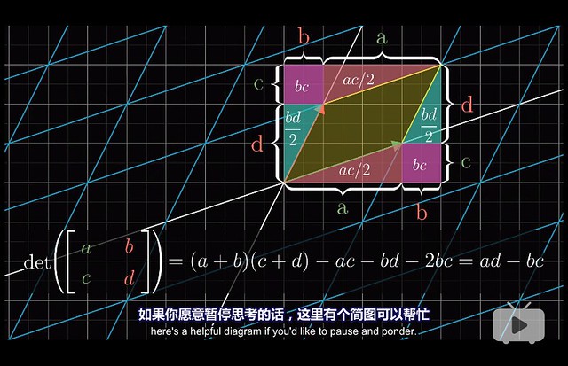
Chapter 5 - The determinant (行列式)
The purpose of computation is insight, not numbers. ―Richard Hamming
Among those linear transformations, some of them seemed to stretch space out, while others squash it in. One thing that turns out to be pretty useful for understanding one of these transformations is to measure exactly how much it stretches or squashes things. More specificantly, to measure the factor by which the area of a given region increases or decreases.
比如 $\icol{3 & 0 \newline 0 & 2}$ 就是把 $\hat i$ 拉伸 3 倍、$\hat j$ 拉伸 2 倍,这样每个网格的面积就变成了原来的 6 倍。(这个面积的计算依赖于我们的前提:”keeping grid lines parallel and evenly spaced”,你试想一下如果变换后变曲线了,面积就不好算了)
This very special scaling factor is called the determinant of that transformation.
If the determinant of a 2-D transformation is 0, it squashes all of space onto a line, or even a single point. Since then, the area of any region would become 0.
However, in fact, a determinant can be negative. How could you scale an area by a negative amount? This has to do with the idea of orientation. Any transformation that turn over the area (想象把一张纸从正面翻到背面) is said to invert the orientation of space.
Another way to think about it is to consider $\hat i$ and $\hat j$. Notice that in their starting positions, $\hat j$ is to the left of $\hat i$ ($\hat j$ 在沿 $\hat i$ 剪开的左半边). If after transformation, $\hat j$ is on the right of $\hat i$, the orientation of space has been inverted.
Whenever the orientation of space is inverted, the determinant will be negative, but its absolute value still tells you the factor by which the area have been scaled.
If the determinant of a matrix is 0, the basis vectors inside this matrix are linearly depenedent.
Chapter 6 - Inverse matrices, column space, rank and null space (kernel)
To ask the right question is harder than to answer it. ―Georg Cantor
The main reasons that linear algebra is more broadly applicable and required for just about any technical discipline is that it let us solve certain systems of equations. By “systems of equations”, I mean you have a list of variables and a list of equations relating them.
线性方程组即是 linear system of equations.
To solve $A \vec x = \vec v$ is equivalent to, given linear transformation $A$, look for a vector $\vec x$, which lands on $\vec v$ after applying the transformation.
Let’s start with $\operatorname{det}(A) \neq 0$.
Applying the transformation on $\vec x$ in reverse is equivalent to applying the inverse of $A$ onto $\vec v$.
\[\vec x = A^{-1} \vec v\] \[A^{-1}A = I\]But when $\operatorname{det}(A) = 0$, there is no inverse of $A$ (i.e. $A^{-1}$ does not exist). You cannot “unsquash” a line into a plane. At least that’s not something a function can do because that would require transforming each individual vector on the line into a bunch of vectors on that plane but a function can only take a single input to a single output.
However, solution can still exist when $\operatorname{det}(A) = 0$. E.g. if your transformation $A$ squashes the space into a line and you’re lucky that $\vec v$ lives on that line.
You might notice that some of those zero determinant cases feel a lot more restrictive than others (有的是降二维有的只降一维). When the output of a transformation is a line, i.e. 1-D, we say the transformation has a rank of 1. So the rank of a matrix is the number of dimensions in the output of the transformation.
The set of all possible outputs from a matrix, is called the column space of the matrix. In other words, the column space is the span of the columns of the matrix. So a more precise definition of rank would be that it’s the number of dimensions in the column space.
When its rank is equal to the number of columns, we call a matrix full rank.
Note that $\icol{0 \newline 0}$ is always in the column space since linear transformations must keep the origin fixed in place. For a full rank transformation $A$, the only vector $\vec x$ that lands at the origin is the zero vector itself, but for a matrix $A’$ that are not full rank, which squash to a smaller dimension, you can have a whole bunch of vectors $\lbrace \vec{x’} \rbrace$ that land at the origin (比如 2-D 压缩到 1-D 就会有一条直线上的所有 vectors 被压缩到原点;3-D 压缩到 1-D 是有一整个平面上的 vectors 被压缩到原点). This set of vectors $\lbrace \vec{x’} \rbrace$ that lands on the origin is called the null space or the kernel of matrix $A’$. In terms of the linear system of equations, when $\vec v$ happens to be the zero vector, the null space of $A$ gives you all the possible solutions to $A \vec x = \vec v$.
反过来我们可以定义:The null space of matrix $A$ is the set of all vectors $\vec v$ such that $A \vec v = \vec 0$
Chapter 6 Supplement - Nonsquare matrices as transformations between dimensions
首先只有 square matrix 才有 determinant。
A $3\times2$ matrix $A=\icol{a & b \newline c & d \newline e & f}$ would transform a 2-D vector $\vec x=\icol{x_1 \newline x_2}$ in 2-D space into a 3-D vector in 3-D space. 原来 2-D space 里的两个 2-D basis, $\icol{1 \newline 0}$ 和 $\icol{0 \newline 1}$, 现在变成了两个 3-D basis, $\icol{a \newline c \newline e}$ 和 $\icol{b \newline d \newline f}$。但是正常 3-D space 应该有 3 个 3-D basis vector,这说明 $A$ 的 column space 只可能是这个 3-D space 中的一个 plane。
A $2\times3$ matrix $A=\icol{a & b & c \newline d & e & f}$ would transform a 3-D vector $\vec x=\icol{x_1 \newline x_2 \newline x_3}$ in 3-D space into a 2-D vector in 2-D space. 原来 3-D space 里的三个 3-D basis, $\icol{1 \newline 0 \newline 0}$、$\icol{0 \newline 1 \newline 0}$ 和 $\icol{0 \newline 0 \newline 1}$, 现在变成了三个 2-D basis, $\icol{a \newline d}$、$\icol{b \newline e}$ 和 $\icol{c \newline f}$。虽然 2-D space 不需要 3 个 basis,但是不妨碍你用 3 个 basis 来 span 这个 2-D space。
Chapter 7 - Dot products and duality
Let $\vec v = \icol{a \newline b}$, $\vec w = \icol{c \newline d}$ and $\theta$ be the angle between them.
\[\begin{aligned} \vec v \cdot \vec w &= \icol{a \newline b} \cdot \icol{c \newline d} = ac + bd \newline &= (\vec v)^{T} \vec w = (\vec w)^{T} \vec v \newline &= \vert \vec v \vert \times \vert \vec w \vert \times \cos \theta \newline \vert \vec v \cdot \vec w \vert &= (\text{length of projected } \vec v) \times (\text{length of } \vec w) \newline &= (\text{length of projected } \vec w) \times (\text{length of } \vec v) \end{aligned}\]$(\vec v)^{T}$ 是这么一个 transformation:将 2-D space squash 到 1-D 数轴,basis $\icol{1 \newline 0}$ 压到数轴上 $a$ 这个点,basis $\icol{0 \newline 1}$ 压到数轴上 $b$ 这个点,$(\vec v)^{T} \vec w$ 就表示 $\vec w$ 会被压到数轴上 $ac + bd$ 这个点。
反之 $(\vec w)^{T} \vec v$ 也可以这么理解。


Chapter 8 - Cross products
8.1 Standard introduction
非标准定义
$\vert \vec v \times \vec w \vert = \text{Area of parallelogram}$ (以 $\vec v$ 和 $\vec w$ 为两条边的平行四边形的面积). 当 $\vec v$ 在沿 $\vec w$ 切开的左侧时(此时 $\vec w$ 在沿 $\vec v$ 切开的右侧),符号为正;否则符号为负。
$\vec v \times \vec w = -\vec w \times \vec v$
Suppose $\vec v = \icol{a \newline b}$ and $\vec w = \icol{c \newline d}$
$\vec v \times \vec w = \operatorname{det} \big (\icol{a & c \newline b & d} \big )$ (叉乘等于向量合并成的矩阵的 determinant). 令这个合并而成的矩阵为 $A$。
$\because A \hat i = \icol{a & c \newline b & d} \icol{1 \newline 0} = \icol{a \newline b} = \vec v$
$\,\,\,\, A \hat j = \icol{a & c \newline b & d} \icol{0 \newline 1} = \icol{c \newline d} = \vec w$
$\,\,\,\, \text{and } \hat i \times \hat j = 1$
$\therefore \vec v \times \vec w = \operatorname{det}(A) \times (\hat i \times \hat j) = \operatorname{det}(A)$
标准定义
The cross product is not a number, but a vector. $\vec v \times \vec w = \vec p$. The resulted-in vector $\vec p$’s length will be the area of the $vw$ parallelogram, and its direction will be perpendicular (垂直) to that parallelogram. But there are two directions perpendicular to that parallelogram. Here we need the “Right Hand Rule” (右手定则): 右手食指顺着 $\vec v$ 方向,中指顺着 $\vec w$ 方向,大拇指即为 $\vec p$ 的方向。
按这个定义:两个 2-D vectors 不可能求出叉积,虽然你可以按 determinant 来算出一个 scalar。所以一般叉积是指两个 3-D vectors 的叉积。
死记硬背式:$\icol{v_1 \newline v_2 \newline v_3} \times \icol{w_1 \newline w_2 \newline w_3} = \operatorname{det} \big (\icol{\hat i & v_1 & w_1 \newline \hat j & v_2 & w_2 \newline \hat k & v_3 & w_3} \big )$ (这里这个 determinant 得到不是一个 scalar 而是一个由 $\hat i$、$\hat j$ 和 $\hat k$ 表示的 3-D vector)
Digress: dot product 与 cross product 的几何意义
假定我们限定 $\vec v$ 和 $\vec w$ 的长度而不限定它们的方向,那么:
- 令 $p = \vec v \cdot \vec w$,则 $p$ 值的大小代表 $\vec v$ 和 $\vec w$ 共线的程度
- 令 $\vec p = \vec v \times \vec w$,则 $p$ 的长度代表 $\vec v$ 和 $\vec w$ 垂直的程度
8.2 Deeper understanding with linear transformations
考虑 Chapter 7 - Dot products and duality 时我们说过的 $\vec v \cdot \vec w = (\vec v)^{T} \vec w$。The takeaway is that whenever you’re out in the mathematical wild and you find a linear transformation to the number line (数轴), you’ll be able to match it to some vector, which is called the dual vector of that transformation, so that performing the linear transformation is the same as taking a dot product with that dual vector. 比如 transformation $(\vec v)^{T}$ 的 dual vector 就是 $\vec v$。
Our plan:
- Define a 3D-to-1D linear transformation in terms of $\vec v$ and $\vec w$
- Find its dual vector
- Show that this dual vector is $\vec v \times \vec w$
我们注意到:$\operatorname{det} \big (\icol{x & v_1 & w_1 \newline y & v_2 & w_2 \newline z & v_3 & w_3} \big )$ 其实是关于 $\icol{x \newline y \newline z}$ 的一个函数 (这里 $x$、$y$ 和 $z$ 是 scalar,不是前面的 $\hat i$、$\hat j$ 和 $\hat k$;所以这个 determinant 得出来是一个具体值),而且这是一个 3D-to-1D 的 linear transformation。我们就会想知道是否存在一个 dual vector 满足 $\icol{? & ? & ?} \icol{x \newline y \newline z} = \operatorname{det} \big (\icol{x & v_1 & w_1 \newline y & v_2 & w_2 \newline z & v_3 & w_3} \big )$。我们称 $\vec p = \icol{? & ? & ?}^T$,这么一来 $\vec p \cdot \icol{x \newline y \newline z} = \operatorname{det} \big (\icol{x & v_1 & w_1 \newline y & v_2 & w_2 \newline z & v_3 & w_3} \big )$.
Question: what 3-D vector $\vec p$ has the special property that when you take a dot product between $\vec p$ and some other vector $\icol{x \newline y \newline z}$, it gives the same result as if you took the same signed volumn of a parallelepiped (平行六面体) defined by this $\icol{x \newline y \newline z}$ along with $\vec v$ and $\vec w$
Answer: $\vec p = \vec v \times \vec w$
因为 $\vec p$ 的长度等于 $vw$ 平行四边形的面积,且垂直于 $vw$ 平行四边形,然后 $\icol{x \newline y \newline z}$ 到 $\vec p$ 的投影相当于 $\icol{x \newline y \newline z}$-$vw$ 平行六面体的高;所以 $\vec p \cdot \icol{x \newline y \newline z}$ 即是平行六面体的体积,也就是 $\operatorname{det} \big (\icol{x & v_1 & w_1 \newline y & v_2 & w_2 \newline z & v_3 & w_3} \big )$
Chapter 9 - Change of basis (基变换)
Mathematics is the art of giving the same name to different things. ―Henri Poincaré
A space has no grid. 所有的坐标系都是我们人为加上去的。如果一个 vector 用 basis $\hat i$ 和 $\hat j$ 表示为 $\icol{x \newline y}$,那么它在另外一组 basis $\hat{i’}$ 和 $\hat{j’}$ 应该如何表示? (相当于从一个坐标系”翻译”到另外一个坐标系;坐标系的 origin 重合)
假定 $\hat{i’} = \icol{a \newline b}, \hat{j’} = \icol{c \newline d}$,那么 $\icol{a & c \newline b & d} \icol{x’ \newline y’} = \icol{1 & 0 \newline 0 & 1} \icol{x \newline y}$ $\Rightarrow$ 在 $\hat{i’} \hat{j’}$ 坐标系内就应该表示为 $\icol{x’ \newline y’} = \icol{a & c \newline b & d}^{-1} \icol{x \newline y}$
反过来”翻译”的话就是给定 $\icol{x’ \newline y’}$ 然后推出 $\icol{x \newline y} = \icol{a & c \newline b & d} \icol{x’ \newline y’}$
How to translate a matrix?
假定我们在 $\hat i \hat j$ 坐标系下有一个 transformation $M$,那么这个 transformation $M$ 在 $\hat{i’} \hat{j’}$ 坐标系内如何表示?
同理:$\icol{a & c \newline b & d} \big ( M’ \icol{x’ \newline y’} \big ) = \icol{1 & 0 \newline 0 & 1} \big ( M \icol{x \newline y} \big )$ $\Rightarrow$ $M’ \icol{x’ \newline y’} = \icol{a & c \newline b & d}^{-1} \big ( M \icol{x \newline y} \big ) = \icol{a & c \newline b & d}^{-1} \big ( M \icol{a & c \newline b & d} \icol{x’ \newline y’} \big )$
$\therefore M’ = \icol{a & c \newline b & d}^{-1} M \icol{a & c \newline b & d}$
In general, whenever you see an expression like $A^{-1}MA$, it suggests a mathematical sort of empathy (同理心、换位思考、共情). The middle $M$ represents a transformation of some kind as you see it, and the outer two matrices represent the emapathy, the shift in perspective. And the full matrix product represents that same transformation, but as someone else sees it.
Chapter 10 - Eigenvectors and eigenvalues
考虑单个 vector 和它所张成的一条直线。经历一个 linear transformation 之后,有些 vector 会偏离它原来张成的这条直线,有的仍然会留在它自己张成的直线上(只是长度或者方向发生了变化,相当于乘以了一个 scalar)。
All these special vectors that remain on their spans after a lienar transformation are called the eigenvectors of the transformation. Each eigenvector has associated with it, what’s called an eigenvalue, which is just the factor by which it stretched or squashed during the transformation.
With any linear transformation described by a matrix, you could understand what it’s doing by reading off the columns of this matrix as the landing spots for basis vectors. But often a better way to get at the heart of what the linear transformation actually does, less dependent on your particular coordinate system, is to find the eigenvectors and eigenvalues.
作用举例:Consider some 3-D rotation. If you can find an eigenvector for that rotation, what you found is the axis of rotation. (rotation 只旋转不拉伸,eigenvalue 为 1)
公式定义:
\[A \vec v = \lambda \vec v\](现在这个公式看起来多好懂!$\lambda$ 是 eigenvalue,$\vec v$ 是 eigenvector)
求解步骤:
\[\begin{aligned} A \vec v = \lambda I \vec v \newline (A - \lambda I) \vec v = \vec 0 \end{aligned}\]If $\vec v = \vec 0$, it always stands. 如果 $\vec v \neq \vec 0$,我们可以看出 $(A - \lambda I)$ 是一个降维的 transformation,直接把 $\vec v$ squash 到原点,所以我们有 $\operatorname{det}(A-\lambda I) = 0$
A 2-D transformation doesn’t have to have (real) eigenvectors. 即 $\operatorname{det}(A-\lambda I) = 0$ 可能没有实数解。(但 complex eigenvector 和 complex eigenvalue 是存在的,这里不讨论)
如果 $A-\lambda I = 0_{n,n}$ (zero matrix),那么这个 transforamtion 只有一个 eigenvalue $\lambda$,但是所有的 vector 会是 eigenvector。此时 $A = \lambda I$,即只拉伸、不旋转。
What if both basis vectors are eigenvectors? 如果 $A$ 是一个 diagonal matrix,说明所有的 basis vector 都是 $A$ 的 eigenvector,对角线的值都是 eigenvalue。(diagonal matrix 相当于是 n 个 scalar,分别乘以 n 个 basis vector,即拉伸了 n 个 basis vector、并没有旋转)。所以 diagonal matrix 有这么一个特点:$A(A \vec v) = A^2 \vec v, A(A^2 \vec v) = A^3 \vec v, \dots$。
如果我们想利用这一特性计算 $A \cdots A(A \vec v)$,但是 $A$ 并不是 diagonal matrix 该怎么办? If your transformation has a lot of eigenvectors, enough so that you can choose a set of them to span the full space, then you could change your coordinate system so that these eigenvectors are your basis vectors.
假定在 coordinate system $\Theta$ 中, $A$ 的 eigen vector 是 $\icol{a \newline b}$ 和 $\icol{c \newline d}$。以这两个 eigenvector 做 basis 得到新的 coordinate system $\Theta’$,对应的有 transformation $A’ = \icol{a & c \newline b & d}^{-1} A \icol{a & c \newline b & d}$。注意,从 space 的角度来看,$A$ 和 $A’$ 是同一个 linear transformation,只是在不同的 coordinate system 下的表示不同。在 $\Theta’$ 视角下,原 $\Theta$ 下的 $\icol{a \newline b}$ 和 $\icol{c \newline d}$ 这两个 vectors 同样也是 $A’$ 的 eigenvector(只是表示方法还没有变到 $\Theta’$),同时恰好它们又是 $\Theta’$ 的 basis,这就说明 $A’$ 必然是一个 diagonal matrix。所以我们先计算 $A’^{n} \vec{v’}$,然后再”翻译”回 $A \cdots A(A \vec v)$。
(如果没有足够的 eigenvector 能 span the full space,你就拼不出足够的 column 到 $\icol{a & c \newline b & d}$ 去给 $A$ 做 basis change)
Chapter 11 - Abstract vector spaces
Linear transformation for functions
Formal definition of linearity:
- Additivity: $L(\vec v + \vec w) = L(\vec v) + L(\vec w)$
- Scaling: $L(c \vec v) = c L(\vec v)$
“keeping grid lines parallel and evenly spaced” is really just an illustration of what these 2 properties mean in the specific case of points in 2-D space.
Another example: $\frac{d}{dx}$ operator is linear. $\frac{d}{dx}(f(x) + g(x)) = \frac{d}{dx}(f(x)) + \frac{d}{dx}(g(x)), \frac{d}{dx}(c f(x)) = c \frac{d}{dx}(f(x))$
To really drill in the parallele, let’s describe the derivative with a matrix. Let’s limit ourselves on polynomials (i.e. we have a space of all polynomials).
Define basis functions $b_n(x) = x^{n}$. Their roles are similar to $\hat i$, $\hat j$ and $\hat k$ in a 3-D space. Polynomial $a x^2 + bx + c$ can be rewritten as $\icol{c \newline b \newline a \newline \vdots}$. In this way, we can define
\[\frac{d}{dx} = \icol{0 & 1 & 0 & 0 & \cdots \newline 0 & 0 & 2 & 0 & \cdots \newline 0 & 0 & 0 & 3 & \cdots \newline 0 & 0 & 0 & 0 & \cdots \newline \vdots & \vdots & \vdots & \vdots & \ddots }\]注意这个矩阵的第一列相当于 $\frac{d}{dx}(b_0(x))$,第二列相当于 $\frac{d}{dx}(b_1(x))$,etc.
| Linear algebra concepts | Alternative names when applied to functions |
|---|---|
| Linear transformations | Linear operators |
| Dot products | Inner products |
| Cross products | N/A |
| Eigenvectors | Eigenfunctions |
What is a vector?
As long as you’re dealing with a set of objects where there’s a reasonable notion of scaling and adding, whether that’s a set of arrows in apce, list of numbers, functions or whatever you choose to define, all the tools developed in linear algebra regarding vectors, linear transformations and all that stuff, should be able to apply.
Thses sets of vetor-ish things (arrows, lists of numbers, functions, etc) are called vector spaces.
我们有 8 条 rules for vectors addition and scaling:

These rules are called axioms. If a space statisfies these 8 axioms, it is a vector space. Axioms are not rules of nature, but an interface (consider Java Interface!)
The form that your vectors take doesn’t really matter as long as there is some notion of adding and scaling vectors that follow these axioms.
Abstractness is the price of generality.
Comments