Digest of R for Data Science

Part 0 - Overview

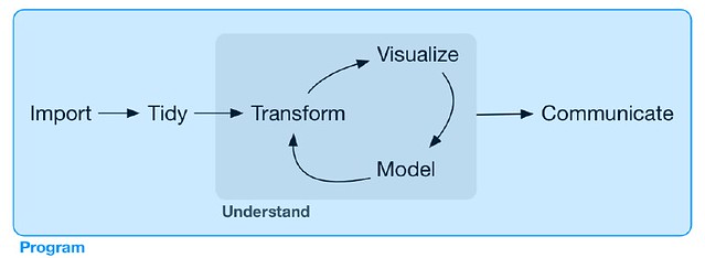
这本书其实主要的内容是 tidyverse。我不知道它为什么加了那么多 R、RStudio 和 Rmd 的内容，而且这本书的编排我是无力吐槽的。总之，这本书掌握 tidyverse 就好。

tidyverse 其实是一个 packages 组合，它的组成部分可以用下面两图概括 (内容其实是一样的，就是觉得图二酷炫一点所以也放上来了)：

Part I - Exploration

Chapter 1 - Data Visualization with ggplot2

data 与 mapping 的完全形式：

ggplot(data = <DATA>， mapping = aes(<MAPPINGS>)) + <GEOM_FUNCTION>(data = <DATA>， mapping = aes(<MAPPINGS>))

ggplot 里的 data 和 mapping 是 plot-global 的，geom 里的 data 和 mapping 是 geom-local 的，你不写就默认全盘使用 global；写了就是在 geom 范围内用 local 覆盖掉 global 相应的部分。这样在有多个 geom 时就可以灵活组合。比如：

ggplot(data = mpg, mapping = aes(x = displ, y = hwy)) +
	geom_point(mapping = aes(color = class)) +
	geom_smooth(data = filter(mpg, class == "subcompact"), se = FALSE)

七参数模型：

ggplot(data = <DATA>) +
    <GEOM_FUNCTION>(mapping = aes(<MAPPINGS>), stat = <STAT>, position = <POSITION>) +
    <COORDINATE_FUNCTION> +
    <FACET_FUNCTION>

The seven parameters in the template compose the grammar of graphics.

Chapter 2 - Workflow: Basics (R 语言基础；略)

Chapter 3 - Data Transformation with dplyr

我要说 Hadley Wickham 真的是取名鬼才。dplyr issue #1857: meaning of dplyr’s name:

The d is for dataframes, the plyr is to evoke pliers (钳子).

And also:

The precursor to dplyr was called plyr. The ‘ply’ in plyr comes from an expansion/refining of the various “apply” functions in R as part of the “split-apply-combine” model/strategy.

本章用的数据集是 nycflights13::flights，需要 library(nycflights13)

3.1 dplyr Basics

• filter(df, x > 1[, y > 2]) 等价于：

  select from df where x > 1 [and y > 2]
  

• arrange(df, x[, y]) 等价于：

  select from df order by x [ASC] [, y [ASC]]
  

• arrange(df, desc(x)[, y]) 等价于：

  select from df order by x DESC [, y [ASC]]
  

• select(df, x[, y]) 等价于：

  select x [, y] from df
  

• select(df, x_prime = x[, y_prime = y]) 等价于：

  select x as x_prime [, y as y_prime] from df
  

• new_df <- mutate(df, xy = x * y) 等价于：

  new_df <- df
  new_df$xy = df$x * df$y
  

• new_df <- transmutate(df, xy = x * y) 等价于：

  new_df <- data.frame()
  new_df$xy = df$x * df$y
  

• summarize():
  • collapse a data frame down to a single row, or
  • collapse a column down to a single value
• All above can be used in conjunction with group_by()

All these functions work similarly:

1. The first argument is a data frame.
2. The subsequent arguments describe what to do with the data frame, using the variable names (without quotes).
3. The result is a new data frame.

3.2 dplyr::filter()

取 (fligths$month == 1) & (flights$day == 1) 的 row：

filter(flights, month == 1, day == 1)  # 多个参数默认是 AND 关系
    # IS EQUIVALENT TO
filter(flights, month == 1 & day == 1)  # 不要用 &&

注意以下符号或函数都可以直接用：

• x & y
• x | y
• !x
• xor(x, y)
• x %in% c(1,2,3)

比如：

filter(flights, month == 11 | month == 12)  # 取 `(fligths$month == 11) | (flights$month == 12)` 的 row；注意不要用 ||
    # IS EQUIVALENT TO
filter(flights, month %in% c(11, 12))

filter(flights, !(arr_delay > 120 | dep_delay > 120))

如果 column 上有 NA 值，那么对应的 row 不会被取到：

df <- tibble(x = c(1, NA, 3))

filter(df, x > 1)
#> # A tibble: 1 x 1
#>       x
#>   <dbl>
#> 1     3
filter(df, is.na(x) | x > 1)
#> # A tibble: 2 x 1
#>       x
#>   <dbl>
#> 1    NA
#> 2     3

• 这是因为当 x = NA 时，x > 1 不可能被 evaluate 为 TRUE (实际会被 evaluate 成 NA)，那么必然也就不会被选到
• 这和当 x = 0 时，x > 1 是 FALSE 所以自然不会被选到是同一个道理

3.3 dplyr::arrange()

Order flights by flights$year, flights$month and flights$day:

arrange(flights, year, month, day)

默认是升序排列 (order by x ASC)。若要降序 (order by x DESC) 排列，需要给 column name 套一个 desc() 函数：

arrange(flights, desc(year))

注意：不管是升序还是降序，NA 值永远排在最后：

df <- tibble(x = c(5, 2, NA))
arrange(df, x)
#> # A tibble: 3 × 1
#>       x
#>   <dbl>
#> 1     2
#> 2     5
#> 3    NA
arrange(df, desc(x))
#> # A tibble: 3 × 1
#>       x
#>   <dbl>
#> 1     5
#> 2     2
#> 3    NA

3.4 dplyr::select()

flights[, c("year", "month", "day")] 可以写成：

select(flights, year, month, day)

然后 column name 竟然支持 slice 操作！比如 year:day 表示 “all columns between year and day (inclusive)”:

select(flights, year:day)

slice 还可以用负号表示 “inverse selection” (反选)，比如 -(year:day) 表示 “all columns except those from year to day (inclusive)”:

select(flights, -(year:day))

• 注意这个符号不是一定要配合 slice 使用，可以单独用在一个 colname 上，比如 select(flights, -year)：选取除了 “year” 之外的所有 column

3.4.1 dplyr::select() helpers

如果你在导入 tidyverse 后 ？select_helpers 你其实会发现有两组文档：

> library(tidyverse)
> ?select_helpers
Help on topic ‘select_helpers’ was found in the following packages:

  Package               Library
  dplyr                 /home/erik/R/x86_64-pc-linux-gnu-library/3.4
  tidyselect            /home/erik/R/x86_64-pc-linux-gnu-library/3.4

这个 tidyselect 包和 dplyr 的关系是：它是 dplyr 的 backend (参 GitHub: tidyverse/tidyselect)。

而 dplyr 的 select helpers (和后面的 colnames context) 有很多接口是直接 delegate 给 tidyselect 的，我们后面会看到。这也说明这里我们可以不用太区分这两个包。

• 我这里提 tidyselect 是因为你 google 函数名经常是搜到 tidyselect 的文档里去了，但是只要你知道它和 dplyr 的关系，看 tidyselect 的文档其实也是一样能理解的

我们直接看 dplyr 的 ?select_helpers：

• Description: These functions allow you to select variables based on their names.
  • starts_with(): starts with a prefix
  • ends_with(): ends with a prefix
  • contains(): contains a literal string
  • matches(): matches a regular expression
  • num_range(): a numerical range like x01, x02, x03.
  • one_of(): variables in character vector.
  • everything(): all variables.
• Usage
  • current_vars()
  • starts_with(match, ignore.case = TRUE, vars = current_vars())
  • ends_with(match, ignore.case = TRUE, vars = current_vars())
  • contains(match, ignore.case = TRUE, vars = current_vars())
  • matches(match, ignore.case = TRUE, vars = current_vars())
  • num_range(prefix, range, width = NULL, vars = current_vars())
  • one_of(..., vars = current_vars())
  • everything(vars = current_vars())
• Arguments
  • match: A string.
  • ignore.case: If TRUE, the default, ignores case when matching names.
  • vars: A character vector of variable names. When called from inside select() these are automatically set to the names of the table.
  • prefix: A prefix that starts the numeric range.
  • range: A sequence of integers, like 1:5
  • width: Optionally, the “width” of the numeric range. For example, a range of 2 gives “01”, a range of 3 gives “001”, etc.
  • ...: One or more character vectors.
• Return Value: An integer vector giving the position of the matched variables.

简单看几个例子：

选取 name 以 “d” 开头的 column：

> select(flights, starts_with("d"))
# A tibble: 336,776 x 5
     day dep_time dep_delay dest  distance
   <int>    <int>     <dbl> <chr>    <dbl>
 1     1      517         2 IAH       1400
 2     1      533         4 IAH       1416

选取 name 以 “y” 结尾的 column：

> select(flights, ends_with("y"))
# A tibble: 336,776 x 3
     day dep_delay arr_delay
   <int>     <dbl>     <dbl>
 1     1         2        11
 2     1         4        20

选取 name 包含 “arr” 的 column：

> select(flights, contains("arr"))
# A tibble: 336,776 x 4
   arr_time sched_arr_time arr_delay carrier
      <int>          <int>     <dbl> <chr>  
 1      830            819        11 UA     
 2      850            830        20 UA

• select(flights, matches(regex)) 这个就是选取 name 符合 regex 的 column
• select(flights, num_range("x", 8:11)) 这个就是选取 name 为 “x8”, “x9”, “x10”, “x11” 的这 4 个 column
• select(flights, one_of(colnames_vec_a, colnames_vec_b)) 这个 one_of 的命名我觉得是最莫名其妙的，其实你看它源代码的意思是：”取 name 在 $\text{colnames_vec_a} \cap \text{colnames_vec_b}$ 这个交集中的 column”
  • Stack Overflow: Why is one_of() called that? 提到说 one_of 的一个 make sense 的使用场景是：我不知道 colnames_vec_a 到底是什么，它可能是用户输入的，可能是另一个 dataframe 的 colnames。我把 colnames_vec_a 拿过来就是想检查一下它里面的 colnames 是不是都合法，然后用来 subset 当前 dataframe 的时候也不会报 key error

> dplyr::one_of
function (..., vars = current_vars()) 
{
    keep <- c(...)
    if (!is_character(keep)) {
        bad("All arguments must be character vectors, not {type_of(keep)}")
    }
    if (!all(keep %in% vars)) {
        bad <- setdiff(keep, vars)
        warn(glue("Unknown variables: ", paste0("`", bad, "`", 
            collapse = ", ")))
    }
    match_vars(keep, vars)
}
<environment: namespace:dplyr>

• select(flights, everything()) 这个就比较简单了，相当于 select * from flights

另外其实还有一个隐藏的:

• select(flights, tidyselect::last_col()) 选取 last column

3.4.2 dplyr::select() colnames context

我们注意到这所有的 helper 函数都有一个参数 vars = current_vars()，根据文档：

vars: A character vector of variable names. When called from inside select() these are automatically set to the names of the table.

所以 current_vars() 的作用是：返回 dataframe df 的 colnames(df)

从这个角度来看，select(flights, current_vars())， select(flights, one_of(current_vars())) 和 select(flights, everything()) 效果是一样的，但是不建议在应用中使用 current_vars() 因为它是给内部机制服务的，而且随着 package 的发展可能会被 deprecate 掉。dplyr: Select variables:

Retired: These functions now live in the tidyselect package as tidyselect::vars_select(), tidyselect::vars_rename() and tidyselect::vars_pull(). These dplyr aliases are soft-deprecated and will be deprecated sometimes in the future.

从源代码来看，current_vars() 是从一个名为 cur_vars_env 的变量中取得 colnames(df) 的；对应的有一个 set_current_vars() 用来赋值 cur_vars_env：

> dplyr::current_vars
function () 
{
    cur_vars_env$selected %||% abort("Variable context not set")
}
<environment: namespace:dplyr>
> dplyr:::set_current_vars
function (x) 
{
    stopifnot(is_character(x) || is_null(x))
    old <- cur_vars_env$selected
    cur_vars_env$selected <- x
    invisible(old)
}
<environment: namespace:dplyr>

• 我习惯叫 colnames context，统计学的 variable 本质就是 column，所以 variable environment 和 colnames context 是一个意思

而且 cur_vars_env 是 dplyr 的一个全局变量，并不是我一开始想象的 “每次调用 dplyr::select 都会生成一个 select 对象来保存 colnames”

所以我们可以猜想 select(flights, starts_with("d")) 的内部过程是这样的：

> dplyr:::set_current_vars(colnames(flights))  # STEP 1: 保存所有 colnames
> dplyr::current_vars()
 [1] "year"           "month"          "day"            "dep_time"      
 [5] "sched_dep_time" "dep_delay"      "arr_time"       "sched_arr_time"
 [9] "arr_delay"      "carrier"        "flight"         "tailnum"       
[13] "origin"         "dest"           "air_time"       "distance"      
[17] "hour"           "minute"         "time_hour" 
> dplyr::starts_with("d")  # STEP 2: 调用 starts_with("d") 返回待取 colnames 的 integer index
[1]  3  4  6 14 16
> dplyr::select_at(flights, dplyr::starts_with("d"))  # STEP 3: 根据 integer index 获取对应的 column
# A tibble: 336,776 x 5
     day dep_time dep_delay dest  distance
   <int>    <int>     <dbl> <chr>    <dbl>
 1     1      517         2 IAH       1400
 2     1      533         4 IAH       1416

3.4.3 Digression: :: 与 :::

细心的你可能已经发现了，dplyr::current_vars() 用的是 :: 而 dplyr:::set_current_vars 用的是 :::。

这个问题在 Re: [R] How to export a function from a package and access it only by specifying the namespace? 有讲：

…you did not export my_test_f in your NAMESPACE file. To access unexported functions, you must use the ::: operator…

The purpose of the :: operator is for those cases where multiple packages are loaded that each export a function with the same name. This is known as “masking” and the last loaded package will contribute the dominant function–i.e. the function the gets called when the user types functionName() and not packageName::functionName(). The :: operator allows the selection of functions that are masked by the dominant function.

If you really want to conceal a function from user-level code, don’t export it and it will only be accessible via the ::: operator.

• 所以 R 的 NAMESPACE file 大抵相当于 python 的 __all__ (参 Python: __all__)
• 若 functionName 出现在 packageName 的 NAMESPACE file，说明它随着 packageName 被 export，它可以在 library(packageName) 之后被直接访问到或是通过 “双冒号式” packageName::functionName 访问到
• 若 functionName 没有出现在 packageName 的 NAMESPACE file，说明它没有被 export，直接通过函数名或是 “双冒号式” 都无法访问到，但是可以通过 “三冒号式” packageName:::functionName 强行访问到

更多关于 NAMESPACE file 的内容可以参考 Making Your First R Package

3.5 Digression: dplyr::rename() 与 dplyr::select() 与 Named Arguments

• rename(df, x_prime = x[, y_prime = y])：将 column x 重命名为 x_prime
• select(df, x_prime = x[, y_prime = y]) 等价于：

  select x as x_prime [, y as y_prime] from df
  

这种 named arguments 可以用 !!! 来 unpack，类似于 python **dict 的用法。具体参 R: Quasiquotation - Section 6. Unpacking Named Arguments in dplyr

> vars <- c(var1 = "cyl", var2 = "am")
> dplyr::select(mtcars, !!!vars)
                    var1 var2
Mazda RX4              6    1
Mazda RX4 Wag          6    1
Datsun 710             4    1
...                    .    .

3.6 dplyr::mutate() 与 dplyr::transmutate()

• dplyr::mutate()：保留原有 dataframe，根据 column-wise 的运算添加新的 column
• dplyr::transmutate()：只保留新添加的 column，原有 dataframe 的 column 弃用

> flights_sml <- select(flights, year:day, ends_with("delay"), distance, air_time)
> mutate(flights_sml, gain = dep_delay - arr_delay, speed = distance / air_time * 60)
# A tibble: 336,776 x 9
    year month   day dep_delay arr_delay distance air_time  gain speed
   <int> <int> <int>     <dbl>     <dbl>    <dbl>    <dbl> <dbl> <dbl>
 1  2013     1     1         2        11     1400      227    -9  370.
 2  2013     1     1         4        20     1416      227   -16  374.
> transmute(flights_sml, gain = dep_delay - arr_delay, speed = distance / air_time * 60)
# A tibble: 336,776 x 2
    gain speed
   <dbl> <dbl>
 1    -9  370.
 2   -16  374.

column-wise 的 opeartor 包括：

• Logical comparisons: <, <=, >, >=, !=, and ==
• Arithmetic operators: +, -, *, /, ^
• Modular arithmetic: %/% (integer division) and %% (remainder)
• Logs: log(), log2(), log10()
• Offsets: lead() and lag()
• Cumulative and rolling aggregates: cumsum(), cumprod(), cummin(), cummax()， cummean()
• Ranking: min_rank(), row_number(), dense_rank(), percent_rank(), cume_dist(), ntile()
  • 可配合 desc() 使用

3.7 dplyr::summarize()

你写 dplyr::summarise() 也是 OK 的。它的作用是：

• Collapse a column down to a single value
• Collapse a data frame down to a single row

> dplyr::summarize(flights, mean_dep_delay = mean(dep_delay, na.rm = TRUE), mean_arr_delay = mean(arr_delay, na.rm = TRUE))
# A tibble: 1 x 2
  mean_dep_delay mean_arr_delay
           <dbl>          <dbl>
1           12.6           6.90

一般的 aggregation function obey the usual rule of missing values: if there’s any missing value in the input, the output will be a missing value. 所以它们一般都提供 na.rm 这个参数。

常用的 summary functions：

• Measures of location: mean(x), median(x)
• Measures of spread: sd(x), IQR(x) (interquartile range), mad(x) (median absolute deviation)
• Measures of rank: min(x), quantile(x, 0.25), max(x)
• Measures of position: first(x), nth(x, 2), last(x)
• Counts: n(x), n_distinct(x), sum(!is.na(x)), sum(x > 10), mean(y > 0)

3.8 dplyr::group_by()

需要注意的是，dplyr::groupby(df, x, y, z) 返回的仍然是一个 tibble dataframe，它的 grouping 信息 (比如每个 group 的 index) 是隐藏在 dataframe 的 attribute 里的。我们称这个 dataframe 为 grouped dataframe。dplyr 遇到 grouped dataframe 的时候会自动转成 group-wise operation。比如：

> daily <- group_by(flights, year, month, day)  # daily is now a grouped dataframe
> filter(flights, arr_delay > 0)  # 得到的仍然是一个 grouped dataframe
# A tibble: 133,004 x 19
    year month   day dep_time sched_dep_time dep_delay arr_time sched_arr_time arr_delay
   <int> <int> <int>    <int>          <int>     <dbl>    <int>          <int>     <dbl>
 1  2013     1     1      517            515         2      830            819        11
 2  2013     1     1      533            529         4      850            830        20

一般对 grouped dataframe 做 filter 或 mutate 操作，仍然会得到一个相同 level 的 grouped dataframe。例外的是 summary：

When you group by multiple variables, each summary peels off one level of the grouping.

打个比方，你 daily <- group_by(flights, year, month, day) 是一个 3-leveled grouped dataframe，你用了 summary(daily, ...)，每个 group 从 dataframe 坍塌成 row，那么 dplyr 会自动将结果重组成一个 group_by(flights, year, month) 这个级别的 2-leveled grouped dataframe。这个操作可以按 level 递进，比如：

> daily <- group_by(flights, year, month, day)
> n_per_day <- summarise(daily, flights = n())  # 每天的航班数
#> # Groups:   year, month [?]
#>    year month   day flights
#>   <int> <int> <int>   <int>
#> 1  2013     1     1     842
#> 2  2013     1     2     943
> n_per_month <- summarise(n_per_day, flights = sum(flights))  # 每月的航班数
#> # A tibble: 12 x 3
#> # Groups:   year [?]
#>    year month flights
#>   <int> <int>   <int>
#> 1  2013     1   27004
#> 2  2013     2   24951
> n_per_year <- summarise(n_per_month, flights = sum(flights))  # 每年的航班数
#> # A tibble: 1 x 2
#>    year flights
#>   <int>   <int>
#> 1  2013  336776

如果想把 grouped dataframe restore 成 normal 的 dataframe，可以用 ungroup()

Detour: Chapter 14 - Pipes with magrittr

14.1 Direct Pipe: %>%

%>% 来自 magrittr package，它也是 tidyverse 的一部分，所以不需要你显式 import。

考虑下面的应用场景：

df_0 <- read_data(...)

df_1 <- func_1(df_0, ...)
df_2 <- func_2(df_1, ...)
df_3 <- func_3(df_2, ...)

我们可能会想去写一个大的 function 来整合这个繁琐的过程：

func_123 <- function(df_0) {
    df_1 <- func_1(df_0, ...)
    df_2 <- func_2(df_1, ...)
    df_3 <- func_3(df_2, ...)
    return(df_3)
}

我觉得你应该不会用这种写法：

func_123 <- function(df_0) {
    df_3 <- func_3(func_2(func_1(df_0, ...), ...), ...)
    return(df_3)
}

%>% 使用的是第一种思想，而且它的设计意图是：让你只关注 verb (函数名) 而忽略 noun (中间或临时变量名)，比如：

df_0 <- read_data(...)

df_3 <- df_0 %>% 
            func_1(...) %>%  # get df_1
            func_2(...) %>%  # get df_2
            func_3(...)      # get df_3

• 其实有点像 java builder 模式的写法

magrittr 内部的实现大概是：

df_0 <- read_data(...)

func_123 <- function(.) {
    . <- func_1(., ...)
    . <- func_2(., ...)
    . <- func_3(., ...)
    return(.)
}

df_3 <- func_123(df_0)

有两类函数在使用 pipe 时需要额外小心：

• 默认使用 current environment 的函数，比如 assign。因为 %>% 会创建一个 temporary envrionment，%>% 内的 assign 会 get 到这个 temporary environment，那么你的 assign 创建的 variable 就会被 bound 到这个 temporary envrionment。等 %>% 结束，temporary envrionment is out of scope，你的 assign 相当于什么都没有做。此时正确的做法是：把你需要用的 environment 显式传进去而不是让 assign 去获取 current environment：

  > assign("x", 10)  # Assign in .GlobalEnv
  > x
  [1] 10
  > "x" %>% assign(99)  # WRONG! `x` will not be changed in .GlobalEnv
  > x
  [1] 10
  > "x" %>% assign(99, .GlobalEnv)  # OK! 
  > x
  [1] 99
  

  • 类似的函数还有 get() 和 load()
• 使用 lazy evaluation 的函数。In R, function arguments are only computed when the function uses them, not prior to calling the function. 所以 func(stmt, ...) 会先进入函数调用的过程，然后再执行 stmt。但是 pipe 是 computes each element in turn，所以 stmt %>% func(...) 会先执行 stmt 在进入函数调用的过程。书上举了一个 tryCatch 的例子，虽然我觉得是个正常人都不会这么写 ()：

  > tryCatch(stop("!"), error = function(e) "An error")  # 先进入 `tryCatch`，然后执行 `stop`
  [1] "An error"
  > stop("!") %>% tryCatch(error = function(e) "An error")  # 先执行 `stop`，然后才进入 `tryCatch`；但此时已经 stop 了
  Error in eval(lhs, parent, parent) : !
  

  • 类似的函数还有 try(), suppressMessages(), suppressWarnings()
  • 但只要你用 stmt %>% func(...) 这种形式，是个函数可能出类似的问题

需要谨慎使用 pipe 的场合：

• redirect 的次数太多 (> 10)，出了问题不好定位，而且代码不好理解

pipe 配上 dplyr 和 ggplot 简直不要太好用：

> diamonds %>% count(cut, clarity)
# A tibble: 40 x 3
   cut   clarity     n
   <ord> <ord>   <int>
 1 Fair  I1        210
 2 Fair  SI2       466
> diamonds %>% count(cut, clarity) %>%
    ggplot(aes(clarity, cut, fill = n)) + geom_tile()

此外可以用匿名函数写法：

mtcars %>%
{ 
  if (nrow(.) > 0)
    rbind(head(., 1), tail(., 1))
  else .
}

14.2 Tee Pipe: %>T%

此外还有 %T>%，它的逻辑是这样的：

• 一般 LHS %>% RHS %>% foo 这么个 pipe，到 foo 这里，它会接收到 RHS
• 而 LHS %>T% RHS %>% foo 是把 LHS 传给 foo，相当于只在 RHS 那里做了个 void 操作，画个图表示的话就是 $\text{LHS} \underset{\text{RHS}}{\top} \text{foo}$

比如下面这个例子：

rnorm(100) %>%
  matrix(ncol = 2) %>%
  plot() %>%
  str()
#>  NULL

得到 NULL 是因为 plot 没有返回值，我们其实应该把 plot 前面一步那个 matrix 传给 str，所以应该写成：

rnorm(100) %>%
  matrix(ncol = 2) %T>%
  plot() %>%
  str()
#>  num [1:50, 1:2] -0.387 -0.785 -1.057 -0.796 -1.756 ...

它的效果是既画了图 (plot) 又输出了 str()

14.3 Exposition Pipe: %$%

If you’re working with LHS functions that don’t have a data frame based API (i.e. do not have a data argument), you might find %$% useful.

%$% exposes the colnames within the LHS object to the RHS expression. Essentially, it is a short-hand for using the with functions.

This is useful when working with many functions in base R. 举例：

mtcars %$%
  cor(disp, mpg)
#> [1] -0.848

• cor() 应该是接受两个 vector 的
• cor() 又不像 dplyr 里的 function 那样可以理解你不带引号的 colname
• 但是你 %$% 一下，它就能理解你是要取 mtcars$disp 和 mtcars$mpg 来做 cor()

14.4 Bidirectional Pipe: %<>%

其实就是个语法糖：

mtcars <- mtcars %>% transform(cyl = cyl * 2)
    # IS EQUIVALENT TO
mtcars %<>% transform(cyl = cyl * 2)

Chapter 4 - Workflow: Scripts (RStudio 基础；略)

老实说我觉得这本书的编排真的很诡异。

Chapter 5 - Exploratory Data Analysis (EDA；略)

Chapter 6 - Workflow: Projects (继续 RStudio 基础；略)

Part II - Wrangle

Chapter 7 - Tibbles with tibble

How should I react when I read the text below? Thank goodness?

If you’re already familiar with data.frame(), note that tibble() does much less: it never changes the type of the inputs (e.g. it never converts strings to factors!), it never changes the names of variables, and it never creates row names.

Creating tibbles:

• as_tibble(iris)
• tibble(x = 1:5, y = 1, z = x ^ 2 + y)
  • tibble() will automatically recyle inputs of length 1 (y above)
  • tibble() allows you to refer to colnames you just created (z above^
• tribble() short for transposed tibble (I am not impressed at all. Thank you. )

  tribble(
  ~x, ~y, ~z,
  #--|--|----
  "a", 2, 3.6,
  "b", 1, 8.5
  )
  #> # A tibble: 2 x 3
  #>   x         y     z
  #>   <chr> <dbl> <dbl>
  #> 1 a         2   3.6
  #> 2 b         1   8.5
  

subset 需注意：

• df$x == df[["x"]] == df[[1]] 得到的都是 vector
• df["x"] 得到是 dataframe
• 可以使用 pipe

df <- tibble(x = runif(5), y = rnorm(5))

# Extract by name
df$x
#> [1] 0.434 0.395 0.548 0.762 0.254
df[["x"]]
#> [1] 0.434 0.395 0.548 0.762 0.254
# Extract by position
df[[1]]
#> [1] 0.434 0.395 0.548 0.762 0.254

# Use pipe
df %>% .$x
#> [1] 0.434 0.395 0.548 0.762 0.254
df %>% .[["x"]]
#> [1] 0.434 0.395 0.548 0.762 0.254
df %>% .[[1]]
#> [1] 0.434 0.395 0.548 0.762 0.254

df["x"]
# # A tibble: 5 x 1
#       x
#   <dbl>
# 1 0.434
# 2 0.395
# 3 0.548
# 4 0.762
# 5 0.254

df %>% .["x"]
# # A tibble: 5 x 1
#       x
#   <dbl>
# 1 0.434
# 2 0.395
# 3 0.548
# 4 0.762
# 5 0.254

Chapter 8 - Data Import with readr

• read_csv(): comma delimited files
• read_csv2(): semicolon delimited files (common in countries where , is used as the decimal place)
• read_tsv(): tab delimited files
• read_delim(): files with indicated delimiter
• read_fwf(): fixed width files
• read_table(): common variation of fixed width files where columns are separated by white space
• read_log(): Apache style log files

后略

Chapter 9 - Tidy Data with tidyr

There are three interrelated rules which make a dataset tidy:

1. Each variable must have its own column.
2. Each observation must have its own row.
3. Each value must have its own cell.

9.1 tidyr::gather() == melt() / tidyr::spread() == cast()

A common problem is a dataset where some of the column names are not names of variables, but values of a variable. 此时可以用 gather():

> table4a
# A tibble: 3 x 3
  country     `1999` `2000`
* <chr>        <int>  <int>
1 Afghanistan    745   2666
2 Brazil       37737  80488
3 China       212258 213766
> table4a %>% gather(`1999`, `2000`, key = "year", value = "cases")
# A tibble: 6 x 3
  country     year   cases
  <chr>       <chr>  <int>
1 Afghanistan 1999     745
2 Brazil      1999   37737
3 China       1999  212258
4 Afghanistan 2000    2666
5 Brazil      2000   80488
6 China       2000  213766

Another problem is an observation which is scattered across multiple rows. 此时应该用 spread():

> table2
# A tibble: 12 x 4
   country      year type            count
   <chr>       <int> <chr>           <int>
 1 Afghanistan  1999 cases             745
 2 Afghanistan  1999 population   19987071
 3 Afghanistan  2000 cases            2666
 4 Afghanistan  2000 population   20595360
 5 Brazil       1999 cases           37737
 6 Brazil       1999 population  172006362
 7 Brazil       2000 cases           80488
 8 Brazil       2000 population  174504898
 9 China        1999 cases          212258
10 China        1999 population 1272915272
11 China        2000 cases          213766
12 China        2000 population 1280428583
> table2 %>% spread(key = type, value = count)
# A tibble: 6 x 4
  country      year  cases population
  <chr>       <int>  <int>      <int>
1 Afghanistan  1999    745   19987071
2 Afghanistan  2000   2666   20595360
3 Brazil       1999  37737  172006362
4 Brazil       2000  80488  174504898
5 China        1999 212258 1272915272
6 China        2000 213766 1280428583

我完全无法理解这两个方法的命名。简单记忆就是：

• gather()：colnames $\Rightarrow$ values，对应 melt()
• spread()：values $\Rightarrow$ colnames，对应 cast()

9.2 tidyr::separate() / tidyr::unite(): 处理包含复合值的 column

复合值比如一个 column 里都是 x|y 这样的值，理论上它应该分开成两个 column，此时可以用 tidyr::separate()。反过来如果你想创建复合值的 column，可以用 tidyr::unite()

> table3
# A tibble: 6 x 3
  country      year rate             
* <chr>       <int> <chr>            
1 Afghanistan  1999 745/19987071     
2 Afghanistan  2000 2666/20595360    
3 Brazil       1999 37737/172006362  
4 Brazil       2000 80488/174504898  
5 China        1999 212258/1272915272
6 China        2000 213766/1280428583
> table3 %>% separate(rate, into = c("cases", "population"))
# A tibble: 6 x 4
  country      year cases  population
* <chr>       <int> <chr>  <chr>     
1 Afghanistan  1999 745    19987071  
2 Afghanistan  2000 2666   20595360  
3 Brazil       1999 37737  172006362 
4 Brazil       2000 80488  174504898 
5 China        1999 212258 1272915272
6 China        2000 213766 1280428583

• By default, separate() will split values wherever it sees a non-alphanumeric character (i.e. a character that isn’t a number or letter)
• If you wish to use a specific character to separate a column, you can pass the character to the sep argument

You’ll notice that cases and population are character columns above. This is the default behaviour in separate(): it leaves the type of the column as is. We can convert the data types using convert = TRUE:

> table3 %>% separate(rate, into = c("cases", "population"), convert = TRUE)
# A tibble: 6 x 4
  country      year  cases population
* <chr>       <int>  <int>      <int>
1 Afghanistan  1999    745   19987071
2 Afghanistan  2000   2666   20595360
3 Brazil       1999  37737  172006362
4 Brazil       2000  80488  174504898
5 China        1999 212258 1272915272
6 China        2000 213766 1280428583

Chapter 10 - Relational Data with dplyr

• inner_join()
• left_join()
• right_join()
• full_join()
• semi_join(df_x, df_y): keeps all observations in df_x that have a match in df_y
• anti_join(df_x, df_y): drops all observations in df_x that have a match in df_y
• intersect(df_x, df_y): return only observations in both df_x and df_y
• union(df_x, df_y): return unique observations in df_x and df_y
• setdiff(df_x, df_y): return observations in df_x, but not in df_y

Chapter 11 - Strings with stringr

注意 stringr 不是 tidyverse 的组成部分，你需要额外 import

stringr is built on top of the stringi package.

All stringr functions start with str_:

• str_length()
• str_c("x", "y") == "xy"
  • str_c("x", "y", sep=",") == "x,y"
  • str_c(c("x", "y"), collapse=",") == "x,y"
  • str_c("A", c(1,2,3), "Z") == c("A1Z", "A2Z", "A3Z")
  • str_c("Happy", if (TRUE) " birthday")
• str_sub(s, start, end): 取 substring 而不是 substitute
• str_to_upper()
• str_sort()
• str_detect(): 检查是否包含子串
• str_count(): 计算子串的个数

太多了就不列全部了。

Chapter 12 - Factors with forcats (略)

注意 forcats 不是 tidyverse 的组成部分，你需要额外 import

Chapter 13 - Dates and Times with lubridate (略)

注意 lubridate 不是 tidyverse 的组成部分，你需要额外 import

Part III - Program

Chapter 14 - Pipes with magrittr (Relocated 到 Chapter 3 和 Chapter 4 之间)

Chapter 15 - Functions (竟然还是 R 语言基础；略)

Chapter 16 - Vectors (竟然还是 R 语言基础；略)

Chapter 17 - Iteration with purrr

• purrr::map() == apply(MAGRIN = 2): apply by column
  • purrr::map() 返回一个 list
  • purrr::map_lgl() 返回一个 logical vector
  • purrr::map_int() 返回一个 integer vector
  • purrr::map_dbl() 返回一个 double vector
  • purrr::map_chr() 返回一个 character vector

> df <- tibble(a = rnorm(10), b = rnorm(10), c = rnorm(10), d = rnorm(10))
> map_dbl(df, mean)
          a           b           c           d 
 0.35728290 -0.09432359  0.15802926  0.25856451 

本章的很多函数用于 list 就是 element-wise 操作，用于 data frame 就是 column-wise 操作。时刻牢记 data frame 的本质是 list 就很好理解了。

17.1 Shortcuts

比如下面这个 map：

models <- mtcars %>% 
  split(.$cyl) %>% 
  map(function(df) lm(mpg ~ wt, data = df))

可以简写为：

models <- mtcars %>% 
  split(.$cyl) %>% 
  map(~lm(mpg ~ wt, data = .))

• 这里 . 指代 current list element (split 得到的 dataframe list 的元素)
• ~ 取代的是前面 function(df) 的部分
• 更详细的解释可以参考 Stack Overflow: What is meaning of first tilde in purrr::map

另外 attribute 可以通过 string 访问，比如下面获取 summary$r.squared 的代码：

models %>% 
  map(summary) %>% 
  map_dbl(~.$r.squared)
#>     4     6     8 
#> 0.509 0.465 0.423

可以写成:

models %>% 
  map(summary) %>% 
  map_dbl("r.squared")
#>     4     6     8 
#> 0.509 0.465 0.423

17.2 Dealing with Failure: purrr::safely() / purrr::possibly() / purrr::quietly()

When you use the map functions to repeat many operations, the chances are much higher that one of those operations will fail. When this happens, you’ll get an error message, and no output. This is annoying: why does one failure prevent you from accessing all the other successes? How do you ensure that one bad apple doesn’t ruin the whole barrel?

purrr::safely() 可以解决这个问题。它的设计哲学是：它本身一个 adverb，接收一个 verb (function)，返回一个 wrapper function (有点 annotation 的意味)。一般的写法是：

handle <- function(...) { ... }
safely_handle <- safely(handle)

safely_handle(...)

这个 wrapper function 会固定返回一个 list of two：

• lst$result is the original result. If there was an error, this will be NULL.
• lst$error is an error object. If the operation was successful, this will be NULL.

而且它还有一个好处在于：它永远不会 throw an error. Never.

类似还有两个 adverb：

• purrr::possibly(): Always succeeds. Simpler than safely(), because you give it a default value to return when there is an error.

  x <- list(1, 10, "a")
  x %>% map_dbl(possibly(log, NA_real_))
  #> [1] 0.0 2.3  NA
  

• purrr::quietly(): Instead of capturing errors, it captures printed output, messages, and warnings

  x <- list(1, -1)
  x %>% map(quietly(log)) %>% str()
  #> List of 2
  #>  $ :List of 4
  #>   ..$ result  : num 0
  #>   ..$ output  : chr ""
  #>   ..$ warnings: chr(0) 
  #>   ..$ messages: chr(0) 
  #>  $ :List of 4
  #>   ..$ result  : num NaN
  #>   ..$ output  : chr ""
  #>   ..$ warnings: chr "NaNs produced"
  #>   ..$ messages: chr(0)
  

17.3 多路 Iteration：purrr:map2() / purrr:pmap() / purrr:invoke_map()

• purrr:map2(lst_x, lst_y, f): 依次调用 f(lst_x[1], lst_y[1]), f(lst_x[2], lst_y[2]), …, f(lst_x[n], lst_y[n])
  • 如果是 purrr:map2(df_x, df_y, f)，那就是依次调用 f(df_x[col_1], df_y[col_1]), f(df_x[col_2], df_y[col_2]), …, f(df_x[col_n], df_y[col_n])
• purrr:pmap() 就是 purrr:map2() 扩展到大于 2 个 input 的版本
• purrr:invoke_map(func_lst, data_lst): 依次调用 func_lst[1](data_lst[1]), func_lst[2](data_lst[2]), …, func_lst[n](data_lst[n])

17.4 Element-wise 的 void 操作：purrr:walk()

purrr:map() 这些都是有返回值的，有时候我们不需要返回值，只是想 iterate 并做 void 操作，比如我有一个 list of paths，我想 iterate 并 mkdir，此时该如何操作？可以用 purrr:walk()：

x <- list(1, "a", 3)

x %>% walk(print)
#> [1] 1
#> [1] "a"
#> [1] 3

17.5 Predicate Functions

“predicate” 即 “谓语”，predicate function 基本就是 boolean function，亦即只返回 single TRUE or FALSE 的 function

• purrr::keep(df, predicate): 返回一个 dataframe，只保留 predicate(col) == TRUE 的 col
• purrr::discard(df, predicate): 返回一个 dataframe，丢弃 predicate(col) == TRUE 的 col

iris %>% keep(is.factor) %>% str()
#> 'data.frame':    150 obs. of  1 variable:
#>  $ Species: Factor w/ 3 levels "setosa","versicolor",..: 1 1 1 1 1 1 1 1 1 1 ...

iris %>% discard(is.factor) %>% str()
#> 'data.frame':    150 obs. of  4 variables:
#>  $ Sepal.Length: num  5.1 4.9 4.7 4.6 5 5.4 4.6 5 4.4 4.9 ...
#>  $ Sepal.Width : num  3.5 3 3.2 3.1 3.6 3.9 3.4 3.4 2.9 3.1 ...
#>  $ Petal.Length: num  1.4 1.4 1.3 1.5 1.4 1.7 1.4 1.5 1.4 1.5 ...
#>  $ Petal.Width : num  0.2 0.2 0.2 0.2 0.2 0.4 0.3 0.2 0.2 0.1 ...

• purrr::some(df, predicate): 类似于 any([predicate(col) for col in df])
• purrr::every(df, predicate): 类似于 all([predicate(col) for col in df])

x <- list(1:5, letters, list(10))

x %>% some(is_character)
#> [1] TRUE

x %>% every(is_vector)
#> [1] TRUE

• purrr::detect(df, predicate): finds the first element where the predicate is true
• purrr::detect_index(df, predicate): finds the first index where the predicate is true

x <- sample(10)
x
#>  [1]  8  7  5  6  9  2 10  1  3  4

x %>% detect(~ . > 5)  # 注意这里的 predicate 是 function(.) { . > 5 }
#> [1] 8

x %>% detect_index(~ . > 5)
#> [1] 1

• purrr::head_while(df, predicate): keep elements from the start while the predicate is true
• purrr::tail_while(df, predicate): keep elements from the end while the predicate is true

x %>% head_while(~ . > 5)
#> [1] 8 7

x %>% tail_while(~ . > 5)
#> integer(0)

17.6 purrr::reduce() and purrr::accumulate()

vs <- list(
  c(1, 3, 5, 6, 10),
  c(1, 2, 3, 7, 8, 10),
  c(1, 2, 3, 4, 8, 9, 10)
)

vs %>% reduce(intersect)
#> [1]  1  3 10

x <- sample(10)
x
#>  [1]  6  9  8  5  2  4  7  1 10  3
x %>% accumulate(`+`)
#>  [1]  6 15 23 28 30 34 41 42 52 55

Part IV - Model

Chapter 18 - Model Basics with modelr (略)

Chapter 19 - Model Building (略)

Chapter 20 - Many Models with purrr and broom (略)

Part V - Communicate

Chapter 21 - R Markdown

21.2 The process of knitr

When you knit the .Rmd file, it is send to knitr, which executes all of the code chunks and creates a new .md document which includes the code and its output. The .md file is then processed by pandoc, which is responsible for creating the finished file.

21.2 Bibliographies and Citations

Need one such line in your YAML header:

bibliography: rmarkdown.bib

To create a citation within your .Rmd file, use a key composed of @ + the citation identifier from the bibliography file. Then place the citation in square brackets. Here are some examples:

Separate multiple citations with a `;`: Blah blah [@smith04; @doe99].

You can add arbitrary comments inside the square brackets: 
Blah blah [see @doe99, pp. 33-35; also @smith04, ch. 1].

Remove the square brackets to create an in-text citation: @smith04 
says blah, or @smith04 [p. 33] says blah.

Add a `-` before the citation to suppress the author's name: 
Smith says blah [-@smith04].

When R Markdown renders your file, it will build and append a bibliography to the end of your document. The bibliography will contain each of the cited references from your bibliography file, but it will not contain a section heading. As a result it is common practice to end your file with a section header for the bibliography, such as # References or # Bibliography.

You can change the style of your citations and bibliography by referencing a .csl (Citation Style Language) file in the csl field:

bibliography: rmarkdown.bib
csl: apa.csl

Chapter 22 - Graphics for Communication with ggplot2

22.1 Annotations

geom_text 的 annotation 效果有点挫：

best_in_class <- mpg %>%
  group_by(class) %>%
  filter(row_number(desc(hwy)) == 1)

ggplot(mpg, aes(displ, hwy)) +
  geom_point(aes(colour = class)) +
  geom_text(aes(label = model), data = best_in_class)

换成 geom_label 稍微好那么一点点：

ggplot(mpg, aes(displ, hwy)) +
  geom_point(aes(colour = class)) +
  geom_label(aes(label = model), data = best_in_class, nudge_y = 2, alpha = 0.5)

用 ggrepel::geom_label_repel 效果明显改善。It will automatically adjust labels so that they don’t overlap：

ggplot(mpg, aes(displ, hwy)) +
  geom_point(aes(colour = class)) +
  geom_point(size = 3, shape = 1, data = best_in_class) +
  ggrepel::geom_label_repel(aes(label = model), data = best_in_class)

22.2 Legend Layout

确定 legend 的位置：

base <- ggplot(mpg, aes(displ, hwy)) +
  geom_point(aes(colour = class))

base + theme(legend.position = "left")
base + theme(legend.position = "top")
base + theme(legend.position = "bottom")
base + theme(legend.position = "right") # the default

可以用 guides() along with guide_legend() or guide_colourbar() 进一步控制 legend 的样式：

ggplot(mpg, aes(displ, hwy)) +
  geom_point(aes(colour = class)) +
  geom_smooth(se = FALSE) +
  theme(legend.position = "bottom") +
  guides(colour = guide_legend(nrow = 1, override.aes = list(size = 4)))
#> `geom_smooth()` using method = 'loess' and formula 'y ~ x'

Chapter 23 - R Markdown Formats (略)

Chapter 23 - R Markdown Workflow (略)